Iron - bcc

This notebook drives the interfacemethod package to predict the melting point of a unary crystal for a given LAMMPS interatomic potential, using the solid-liquid interface method. LAMMPS itself is called through lammpsparser, the individual LAMMPS calls are dispatched locally or to an HPC queue by executorlib, and the on-the-fly structure analysis (common neighbor analysis, Voronoi volumes) uses structuretoolkit.

The notebook has two parts:

• Configuration (below) - a handful of cells you are expected to edit: the interatomic potential and element to use (input.json), where LAMMPS is run from and how it is called, and how many LAMMPS calls should run concurrently.

• Automated protocol (from “From here on the notebook is automated” onward) - runs the interface method end to end and should not need any changes. The markdown headers in that part explain what each step does and, where applicable, how to read the plots it produces.

See the repository README for installation instructions and worked examples.

%matplotlib inline
import json
import os
import random

import numpy as np
import pandas
import pylab as plt
import structuretoolkit as stk
from ase.build import bulk
from ase.data import reference_states, atomic_numbers
from executorlib import SingleNodeExecutor

from interfacemethod import (
    minimize_structure_positions,
    minimize_structure_volume,
    check_diamond,
    analyse_minimized_structure,
    run_npt_step,
    bisection_step,
    initialise_iterators,
    round_temperature_next,
    npt_solid,
    npt_liquid,
    remove_selective_dynamics,
    get_strain_lst,
    run_strain_point,
    plot_solid_liquid_ratio,
    ratio_selection,
    plot_equilibration,
    check_for_holes,
    plot_melting_point_prediction,
    validate_convergence,
)

Configuration

The following cells define the calculation and are the only ones you typically need to edit:

• project_path - working directory the individual LAMMPS calculations are executed in.

• input_file / output_file - the input.json the potential and element are loaded from (if present) and the output.json the melting point prediction and intermediate results are written to, so an interrupted calculation can simply be resumed by rerunning the notebook.

• lmp_command - the command used to invoke LAMMPS, e.g. prefix it with mpirun -n 4 to run every individual LAMMPS call on 4 MPI ranks.

• max_workers - the number of LAMMPS calls executorlib’s SingleNodeExecutor is allowed to run concurrently. Replace SingleNodeExecutor with executorlib.SlurmClusterExecutor or executorlib.FluxClusterExecutor further down to submit the individual LAMMPS calls to an HPC queue instead of running them on the local machine.

• input_dict / potential - the interatomic potential, read from input.json (falling back to a default Al Morse potential for a quick test if no input.json is present).

• project_parameter - the numerical settings of the interface method (number of atoms, run lengths, convergence criteria, …); any key also present in input.json overrides the default defined here.

• the last cell of this section reloads step_dict from output.json if it already exists, so a previous, interrupted run is resumed rather than recomputed from scratch.

project_path = "melting"

input_file = 'input.json'
output_file = 'output.json'

lmp_command = "lmp -in lmp.in"

max_workers = 4

if os.path.exists(input_file) and os.stat(input_file).st_size != 0:
    with open(input_file, 'r') as f:
        input_dict = json.load(f)
else:
    input_dict = {
        "config": [
            "pair_style morse 9.97749\n",
            "pair_coeff * * 0.4174 1.3885 2.845\n"
        ],
        "species": ["Al"],
        "element": "Al"
    }

input_dict

{'config': ['pair_style eam/alloy \n', 'pair_coeff * * Fe-C-Bec07.eam Fe C\n'],
 'filename': 'Fe-C-Bec07.eam',
 'species': ['Fe', 'C'],
 'element': 'Fe'}

input_dict["config"][1] = input_dict["config"][1].replace(input_dict["filename"], os.path.abspath(input_dict["filename"]))
input_dict

{'config': ['pair_style eam/alloy \n',
  'pair_coeff * * /home/jan/projects/pyiron_meltingpoint/examples/bccFe/Fe-C-Bec07.eam Fe C\n'],
 'filename': 'Fe-C-Bec07.eam',
 'species': ['Fe', 'C'],
 'element': 'Fe'}

pot_dict = input_dict.copy()

if 'model' not in pot_dict.keys():
    pot_dict['model'] = 'Lammps'
if 'name' not in pot_dict.keys():
    pot_dict['name'] = 'CustomPotential'
if 'filename' not in pot_dict.keys():
    pot_path = []
else:
    pot_path = [os.path.abspath(pot_dict['filename'])]
potential = pandas.DataFrame({'Config': [pot_dict['config']],
                             'Filename': [pot_path],
                             'Model': [pot_dict['model']],
                             'Name': [pot_dict['name']],
                             'Species': [pot_dict['species']]
                             })

project_parameter = {
    'run_time_steps': 50000,
    'nvt_run_time_steps': 10000,
    'nve_run_time_steps': 10000,
    'temperature_left': 0,
    'temperature_right': 1000,
    'strain_run_time_steps': 1000,
    'convergence_criterion': 1,
    'potential': potential,
    'cpu_cores': 1,
    'enable_h5md': False,
    'points': 21,
    'boundary_value': 0.25,
    'ratio_boundary': 0.25,
    'timestep_lst': [2, 2, 1],
    'fit_range_lst': [0.05, 0.01, 0.01],
    'nve_run_time_steps_lst': [25000, 20000, 50000],
    'number_of_atoms': 8000,
    'seed': 56570,
}

for k in input_dict.keys():
    project_parameter[k] = input_dict[k]

if 'crystalstructure' not in project_parameter.keys():
    project_parameter['crystalstructure'] = reference_states[atomic_numbers[project_parameter['element']]]['symmetry']

if 'seed' not in project_parameter.keys():
    project_parameter['seed'] = random.randint(0,99999)
project_parameter['seed']

56570

# Values from a previous calculation can be inserted here to reproduce the results
step_dict = {}
if os.path.exists(output_file):
    with open(output_file, 'r') as f:
        step_dict_str = json.load(f)
    for k,v in step_dict_str.items():
        step_dict[int(k)] = v
step_dict

{}

From here on the notebook is automated - no change required !

step_count = 0
temperature_next = None
enable_iteration = True
convergence_goal_achieved = False

Build the initial structure

An ASE bulk supercell for project_parameter['element'] in project_parameter['crystalstructure'] is created and repeated until it contains close to number_of_atoms / 2 atoms - the interface method needs both a solid and a liquid half, so the full simulation cell used from Step 2 onward ends up with roughly number_of_atoms atoms once this structure is duplicated along one axis.

• stk.analyse.get_adaptive_cna_descriptors(...) is a quick sanity check that structuretoolkit’s common neighbor analysis (CNA) correctly recognizes the perfect crystal - the automated part of the notebook relies on this same classification to tell the solid and liquid regions of the interface apart later on.

• stk.visualize.plot3d(basis) shows an interactive 3D view of the defect-free solid supercell before any LAMMPS calculation is run, so you can check the structure looks as expected before committing compute time to it.

if 'lattice_constant' in project_parameter.keys():
    a = project_parameter['lattice_constant']
else:
    a = None
if project_parameter['crystalstructure'] == 'hcp':
    basis = bulk(name=project_parameter['element'], crystalstructure=project_parameter['crystalstructure'].lower(), a=a, orthorhombic=True)
else:
    basis = bulk(name=project_parameter['element'], crystalstructure=project_parameter['crystalstructure'].lower(), a=a, cubic=True)
basis_lst = [basis.repeat([i, i, i]) for i in range(5,30)]
basis = basis_lst[np.argmin([np.abs(len(b)-project_parameter['number_of_atoms']/2) for b in basis_lst])]

stk.analyse.get_adaptive_cna_descriptors(basis, ovito_compatibility=True)

{'CommonNeighborAnalysis.counts.OTHER': 0,
 'CommonNeighborAnalysis.counts.FCC': 0,
 'CommonNeighborAnalysis.counts.HCP': 0,
 'CommonNeighborAnalysis.counts.BCC': 4394,
 'CommonNeighborAnalysis.counts.ICO': 0}

stk.visualize.plot3d(basis)

timestep_iter, fit_range_iter, nve_run_time_steps_iter = initialise_iterators(project_parameter)
timestep = next(timestep_iter)
fit_range = next(fit_range_iter)
nve_run_time_steps = next(nve_run_time_steps_iter)

Step 1: set up the solid sample and roughly estimate a melting point

The structure built above is first relaxed with LAMMPS (atomic positions, then cell volume, both at zero pressure) and checked for a diamond lattice, since diamond needs a different CNA classification than bcc/fcc/hcp. estimate_melting_temperature_using_bisection_CNA() then brackets the melting point to within 10 K by repeatedly running NPT MD and using CNA to tell whether the resulting structure is still solid or has already molten.

This step does not produce any plots, it only prints the rough temperature estimate (accurate to roughly ±100 K) that Step 2 below refines into the actual prediction.

with SingleNodeExecutor(cache_directory="cache", max_workers=max_workers) as exe:
    basis_minimize_pos = exe.submit(
        minimize_structure_positions,
        structure=basis, 
        potential=project_parameter["potential"], 
        project_path=project_path,
        lmp_command=lmp_command,
    )
    basis_minimize_vol = exe.submit(
        minimize_structure_volume,
        structure=basis_minimize_pos, 
        potential=project_parameter["potential"], 
        project_path=project_path,
        lmp_command=lmp_command,
    ).result()

diamond_flag = check_diamond(structure=basis_minimize_vol)
diamond_flag

False

(
    structure_after_minimization,
    key_max,
    number_of_atoms,
    distribution_initial_half,
    _,
) = analyse_minimized_structure(structure=basis_minimize_vol)
structure_after_minimization, key_max, number_of_atoms, distribution_initial_half

(Atoms(symbols='Fe4394', pbc=True, cell=[[37.11906294844518, 2.2728870813581253e-15, 2.2728870813581253e-15], [-2.2728870813581253e-15, 37.11906294844518, 2.272887081358126e-15], [-2.2728870813581253e-15, -2.272887081358126e-15, 37.11906294844518]], indices=..., initial_magmoms=..., momenta=...),
 'CommonNeighborAnalysis.counts.BCC',
 4394,
 0.5)

def estimate_melting_temperature_using_bisection_CNA(
    structure,
    potential_dataframe,
    project_path,
    number_of_atoms,
    key_max,
    distribution_initial_half,
    diamond_flag,
    lmp_command,
    max_workers=4,
    temperature_left=0,
    temperature_right=1000,
    run=10000,
    seed=None,
):
    """
    Estimate the melting temperature by bisecting a temperature bracket with NPT MD + CNA:

    1. Run NPT MD at the upper bound of the bracket.
    2. Classify both bracket endpoints as solid- or liquid-dominated (CNA) and narrow the
       bracket towards the phase boundary, running one new NPT MD simulation per step.
    3. Repeat until the bracket is narrower than 10 K.
    """
    structure_left = structure

    # Step 1c-i: NPT MD at the initial upper temperature bound
    structure_right = run_npt_step(
        structure=structure,
        temperature=temperature_right,
        seed=seed,
        potential=potential_dataframe,
        run_time_steps=run,
        project_path=project_path,
        lmp_command=lmp_command,
    )
    temperature_step = temperature_right - temperature_left

    # Step 1c-ii: bisect the bracket until it is narrower than 10 K.
    # Each iteration decides -- from the CNA analysis of the *previous* iteration's structures --
    # which single new NPT MD run to launch next, so unlike the strain scan in Step 2 this loop
    # is inherently sequential and cannot be handed to executor.map(). The parallelizable unit of
    # work at this stage of the workflow is a whole bisection search, e.g. running this function
    # for several elements, potentials or initial seeds concurrently.
    with SingleNodeExecutor(cache_directory="cache", max_workers=max_workers) as exe:
        while temperature_step > 10:
            (
                structure_left,
                structure_right,
                temperature_left,
                temperature_right,
            ) = exe.submit(
                bisection_step,
                number_of_atoms=number_of_atoms,
                key_max=key_max,
                structure_left=structure_left,
                structure_right=structure_right,
                potential=potential_dataframe,
                temperature_left=temperature_left,
                temperature_right=temperature_right,
                distribution_initial_half=distribution_initial_half,
                structure_after_minimization=structure,
                run_time_steps=run,
                seed=seed,
                diamond_flag=diamond_flag,
                project_path=project_path,
                lmp_command=lmp_command,
            ).result()
            temperature_step = temperature_right - temperature_left

    return int(round(temperature_left))

Why this loop is not parallelized. Each bisection step above launches exactly one new NPT MD run, and which temperature it runs at is decided by the CNA classification of the previous step’s structures – iteration N cannot start before iteration N-1 finishes and is analysed. That is different from the strain scan in Step 2, where every strain point starts from the same structure and all points can be dispatched at once.

If you want to use extra compute here, the independent unit of work is a whole bisection search, not a single step within one: for example, estimating the melting point for several elements, potentials, or random seeds at once is embarrassingly parallel across estimate_melting_temperature_using_bisection_CNA() calls, and that outer loop could be handed to a ProcessPoolExecutor/executorlib.Executor the same way the strain scan was.

temperature_next = estimate_melting_temperature_using_bisection_CNA(
    structure=structure_after_minimization,
    potential_dataframe=project_parameter["potential"],
    project_path=project_path,
    number_of_atoms=number_of_atoms,
    key_max=key_max,
    distribution_initial_half=distribution_initial_half,
    diamond_flag=diamond_flag,
    temperature_left=project_parameter["temperature_left"],
    temperature_right=project_parameter["temperature_right"],
    run=project_parameter["strain_run_time_steps"],
    seed=project_parameter['seed'],
    lmp_command=lmp_command,
    max_workers=max_workers,
)
temperature_next

1711

len(structure_after_minimization)

4394

temperature_next   # +/- 100K

1711

if step_count in step_dict.keys():
    temperature_next = step_dict[step_count]['temperature_next']
else:
    step_dict[step_count]= {'temperature_next': temperature_next}

step_dict

{0: {'temperature_next': 1711}}

Step 2: set up the interface structure

run_interface_iteration() builds a solid-liquid interface at the current temperature estimate and refines it into a melting temperature prediction:

1. equilibrate the solid half of the cell at the target temperature (NPT),

2. briefly overheat and re-equilibrate the other half to create a solid-liquid interface (NPT),

3. scan a series of small strains around the current lattice parameter (NVT + NVE), one independent LAMMPS run per strain - this is the parallelization point of the workflow, all strain points are submitted to the executor at once,

4. classify each strain point as solid- or liquid-dominated and keep only the strains where solid and liquid coexist,

5. fit pressure and temperature vs. strain to extrapolate the melting temperature at zero pressure.

With debug_plot=True (the default below) steps 3-5 each produce diagnostic plots, in the order they are generated:

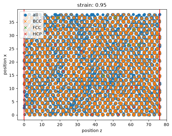
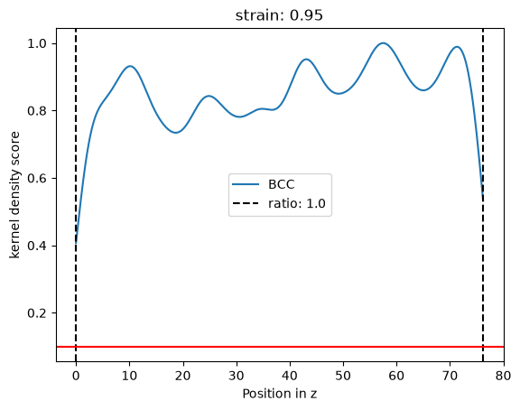
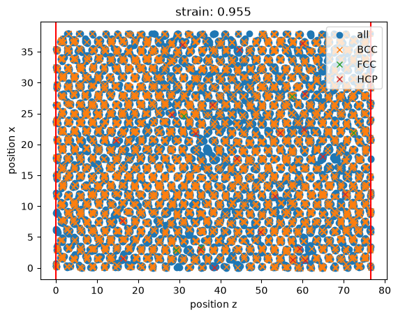
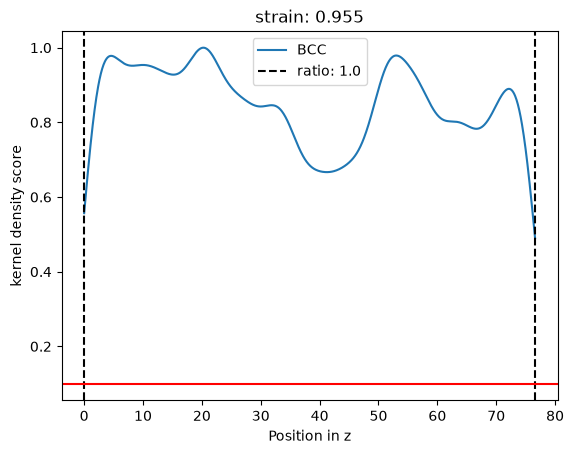
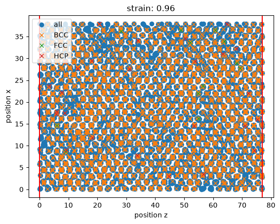
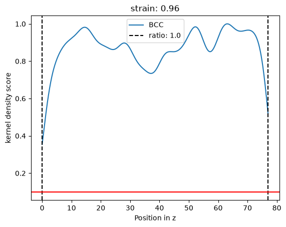
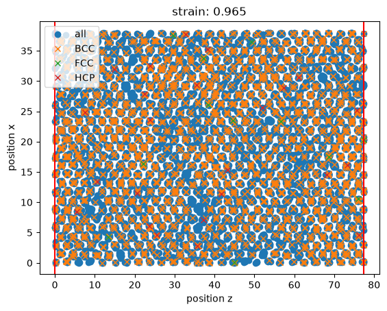
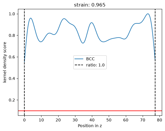
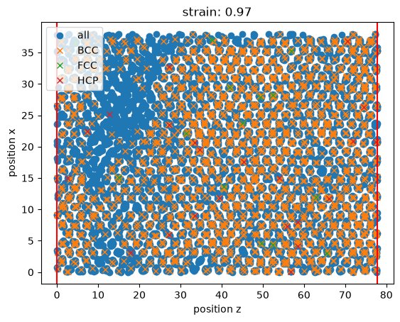
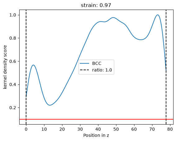
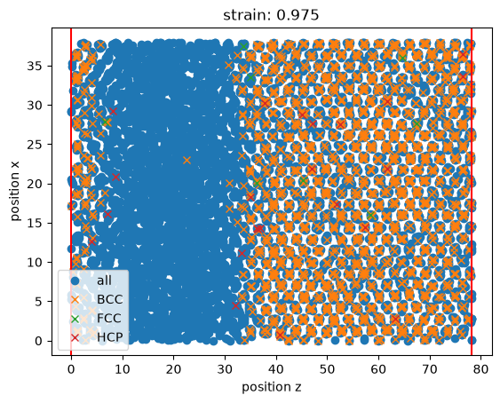
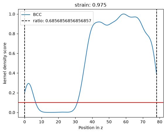
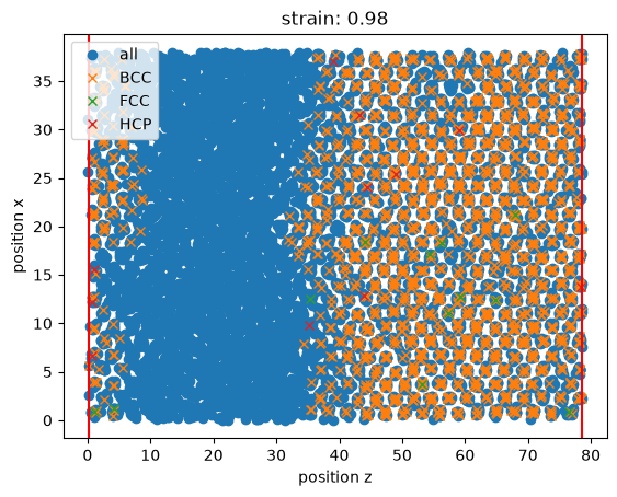
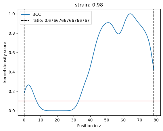
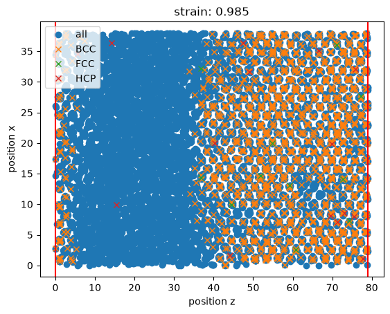
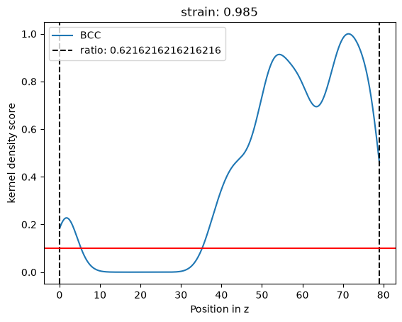
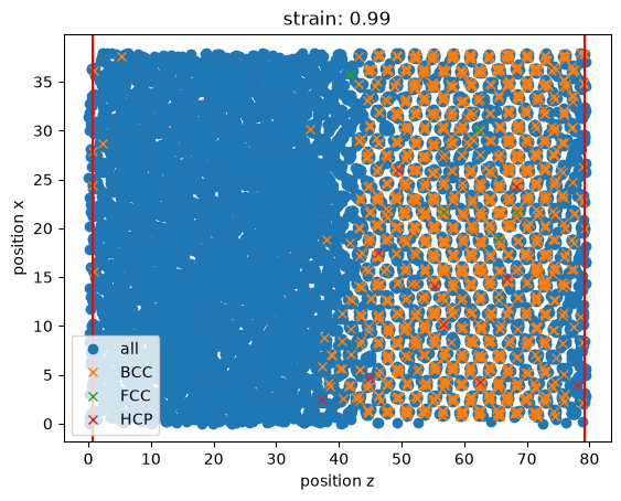
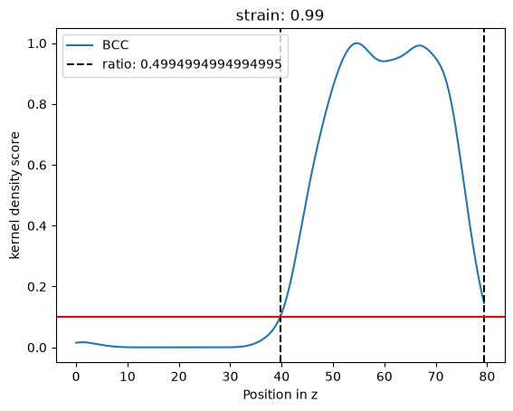
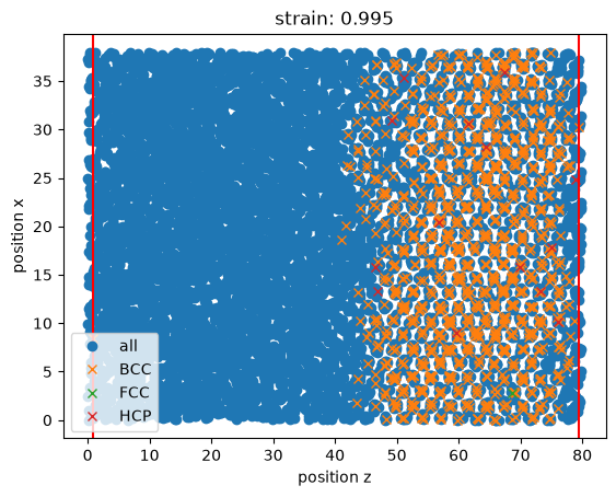
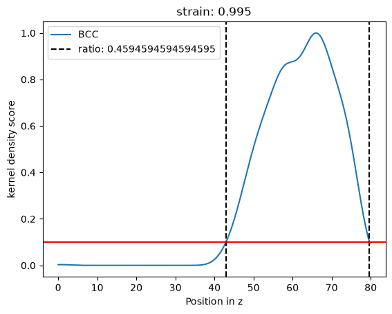
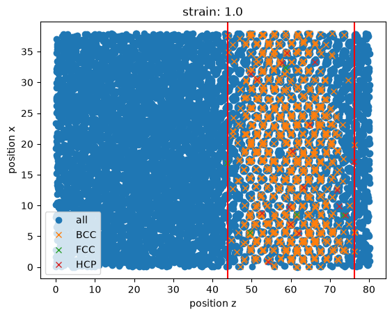
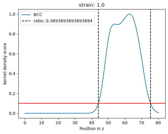
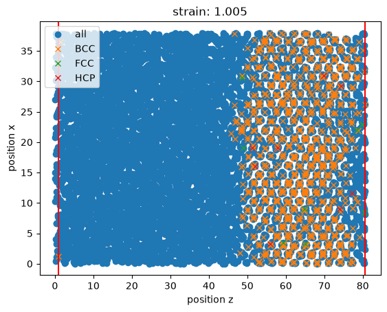
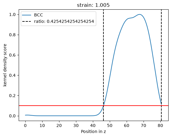
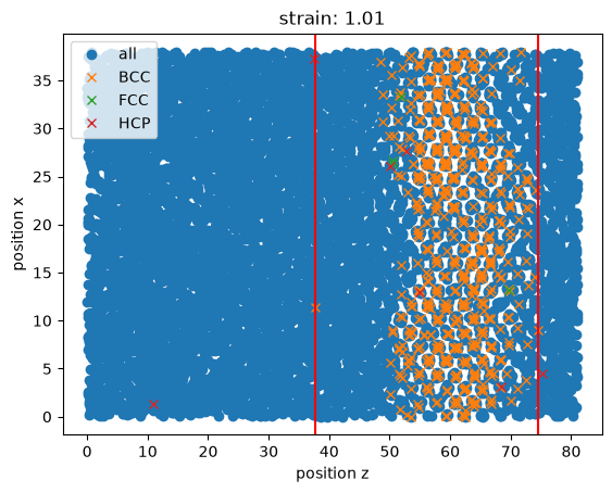
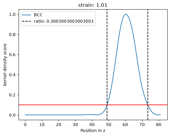
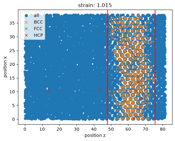
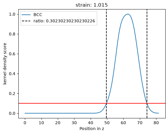
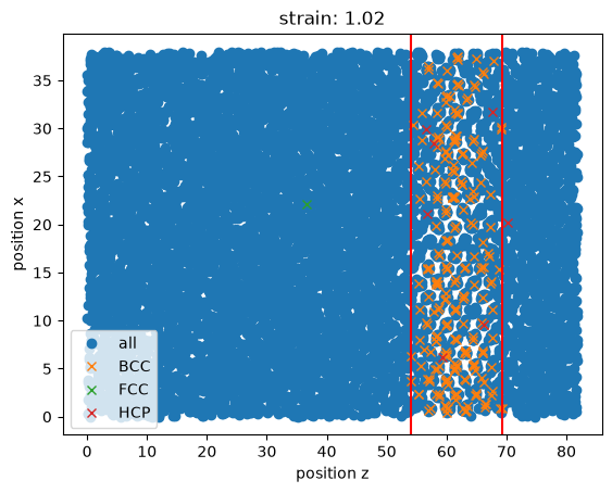
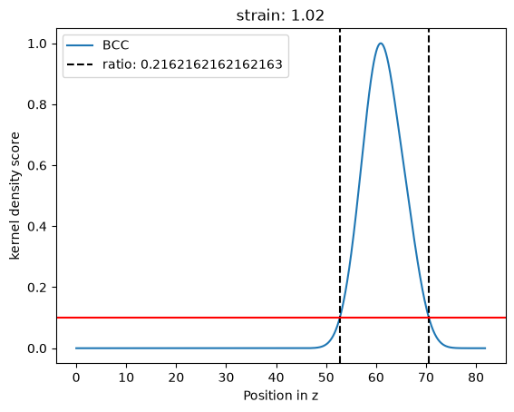
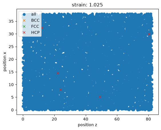
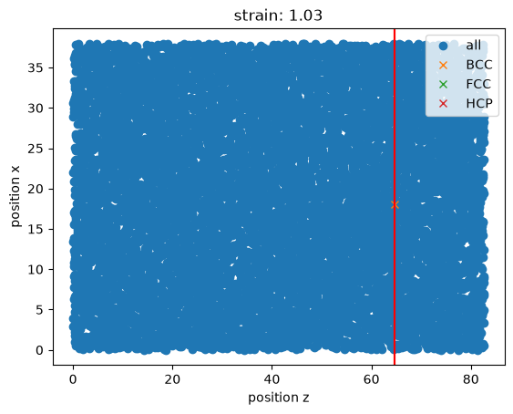
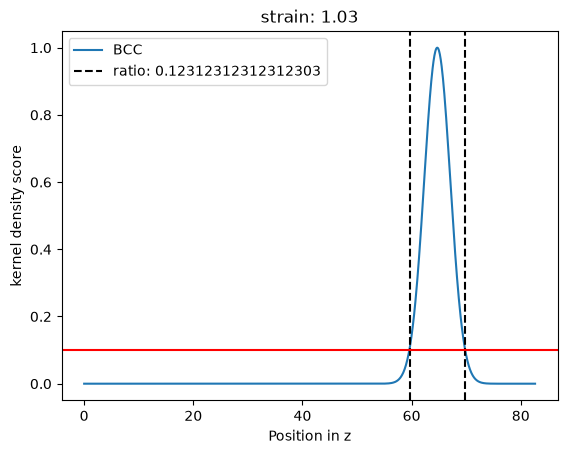
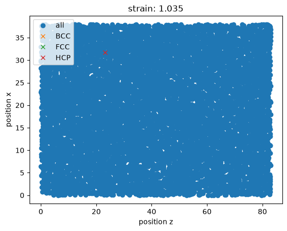
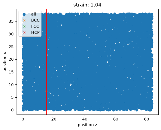
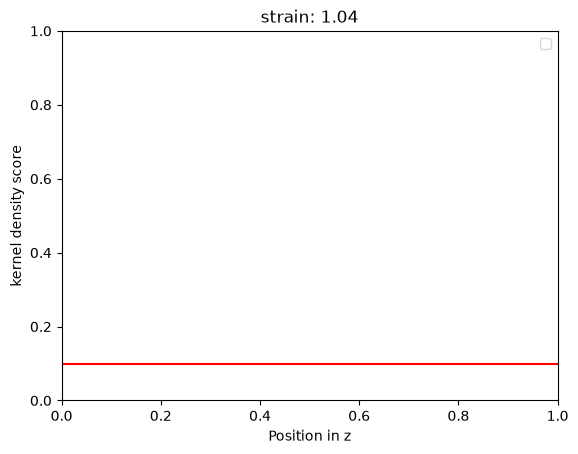
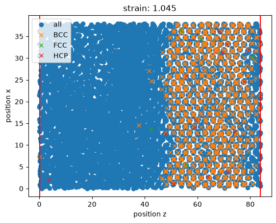
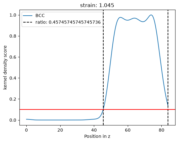
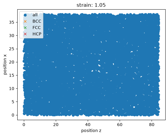
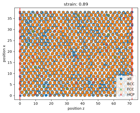
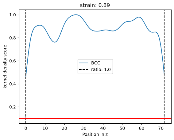
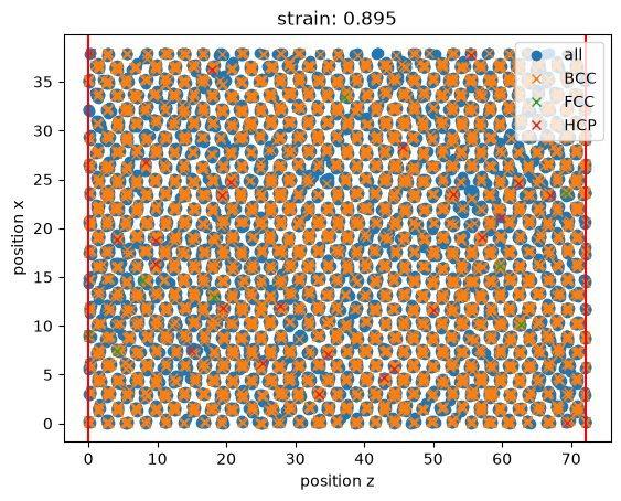
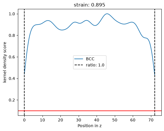
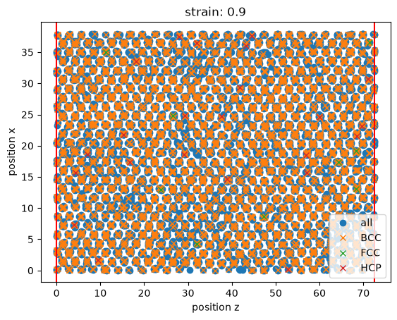
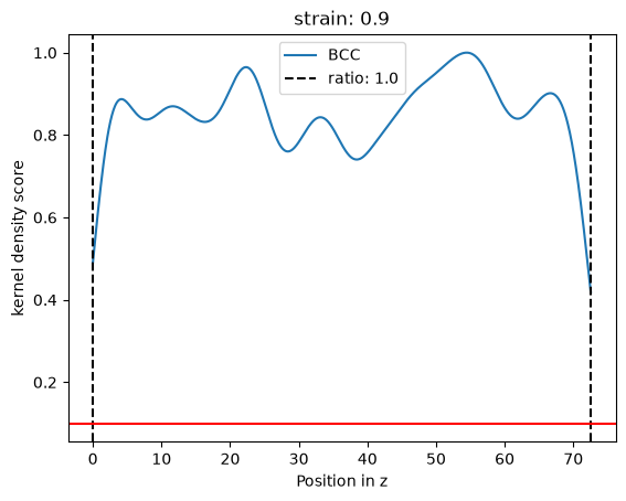
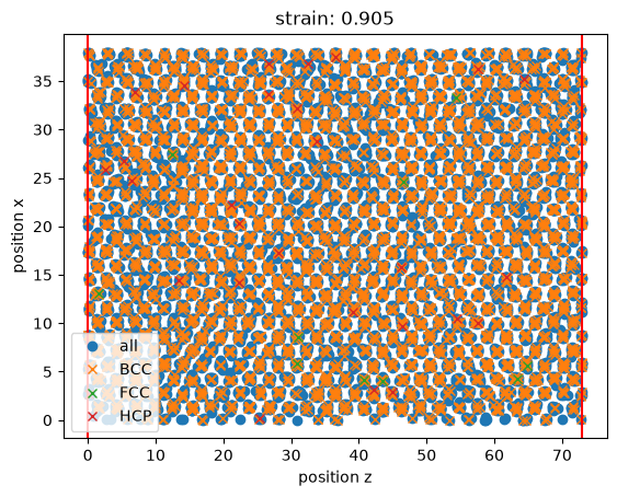
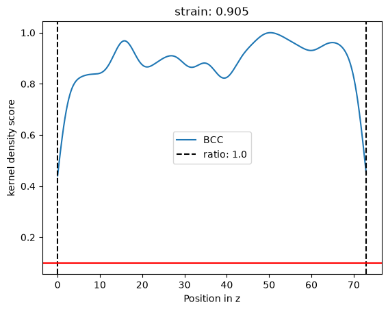
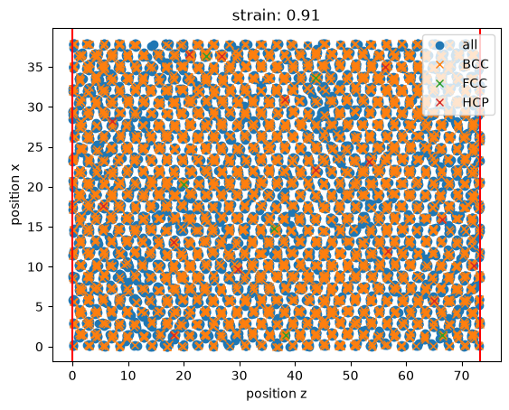
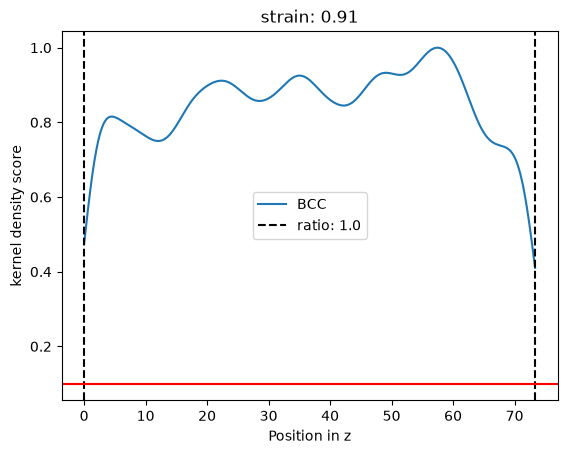
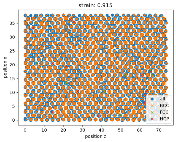
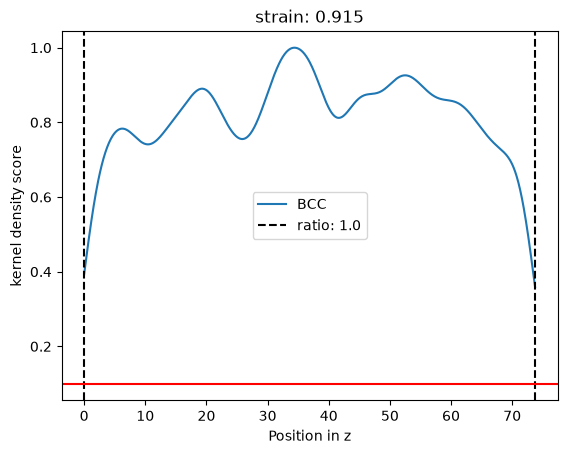
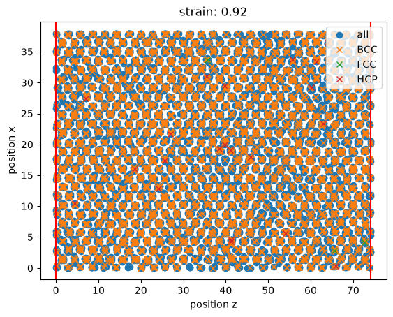
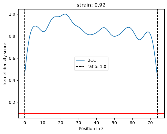
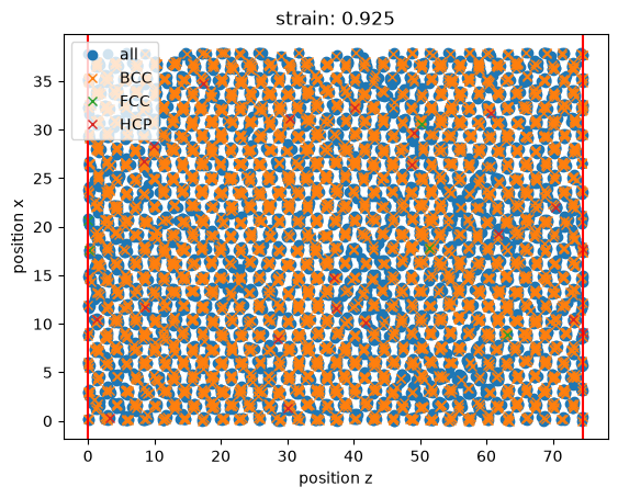
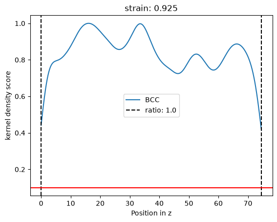
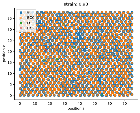
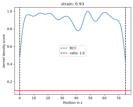
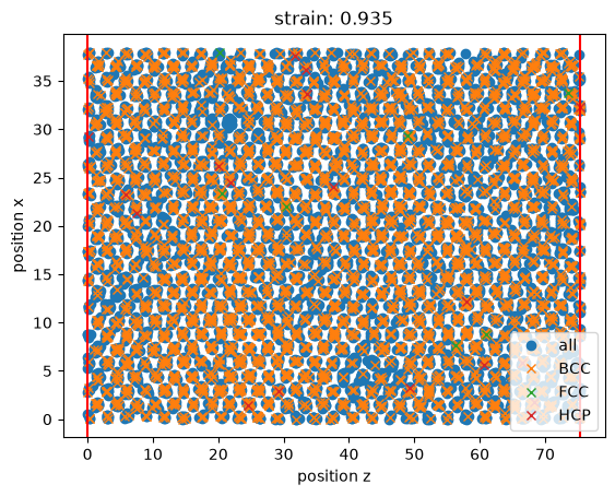
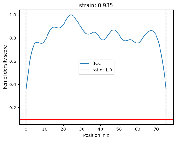
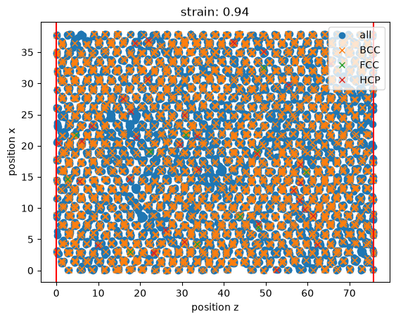
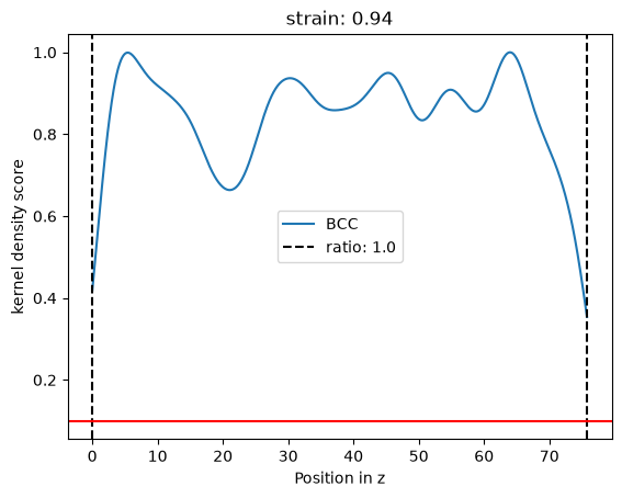
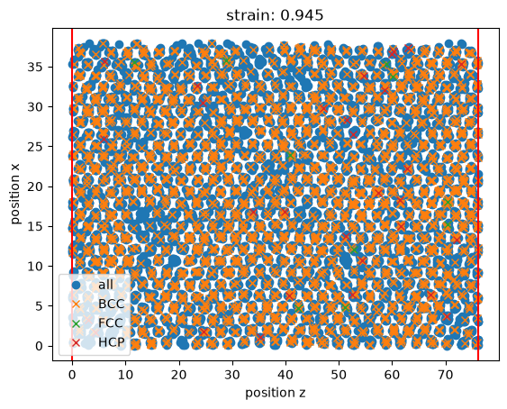
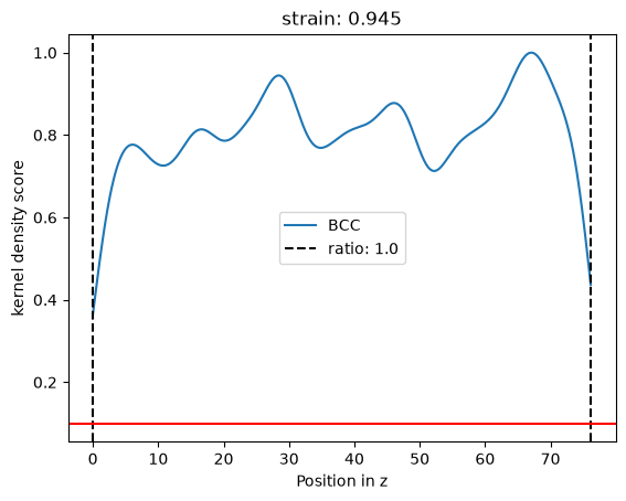
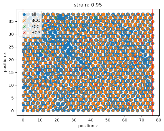
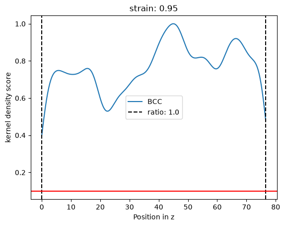
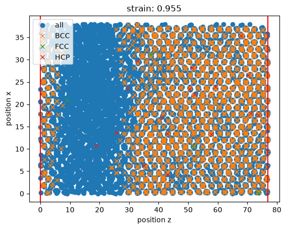
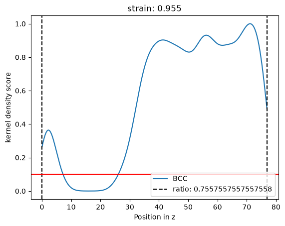
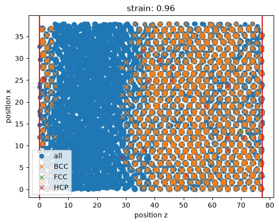
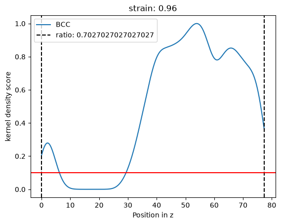
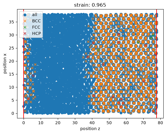
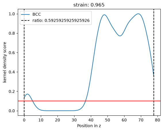
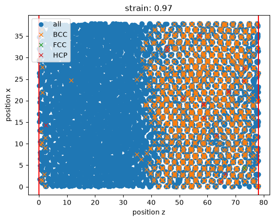
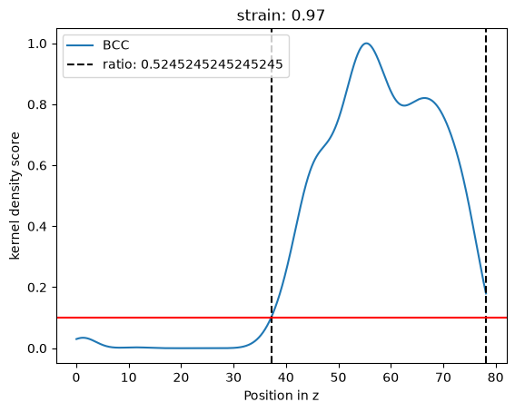
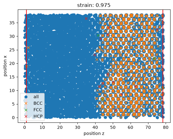
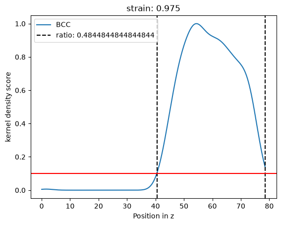
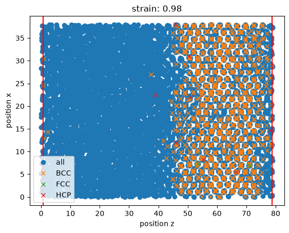
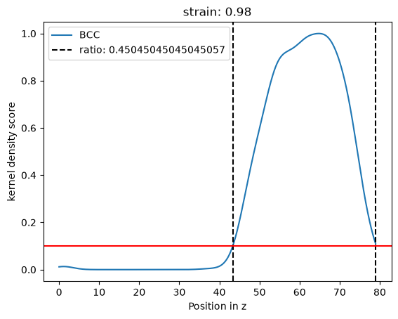
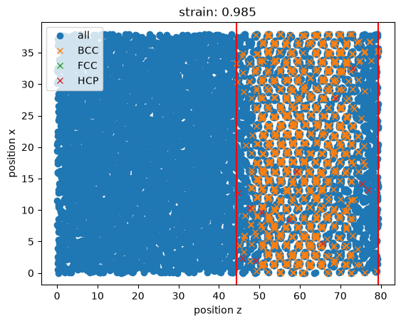
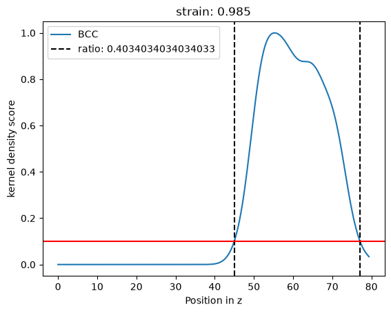
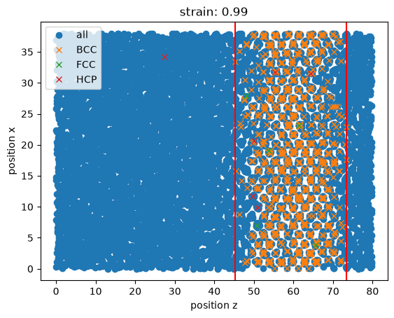
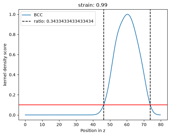
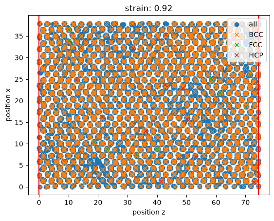
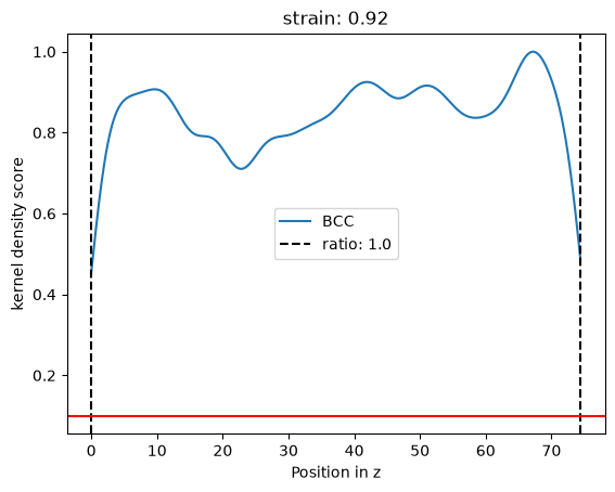
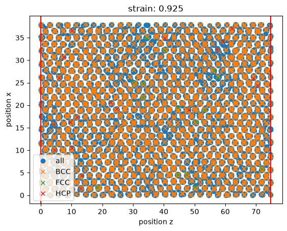
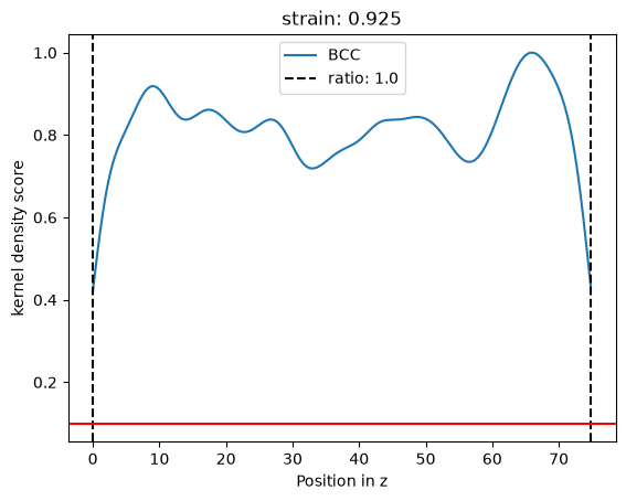
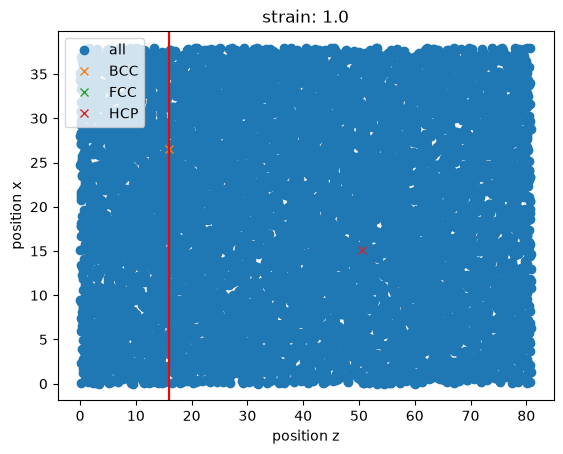
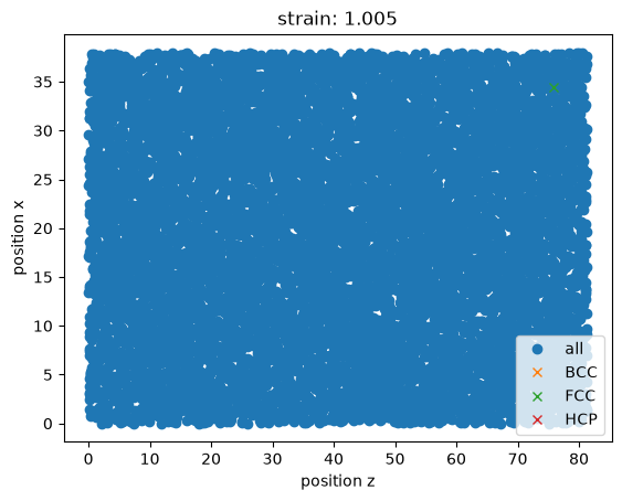
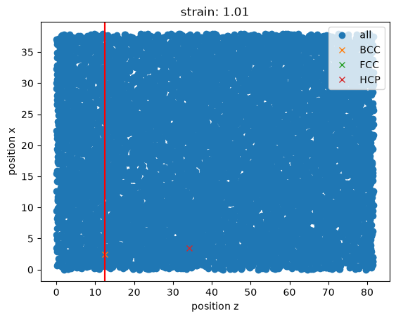
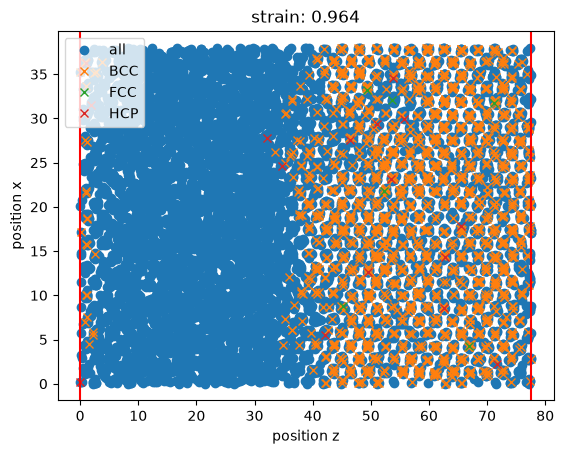
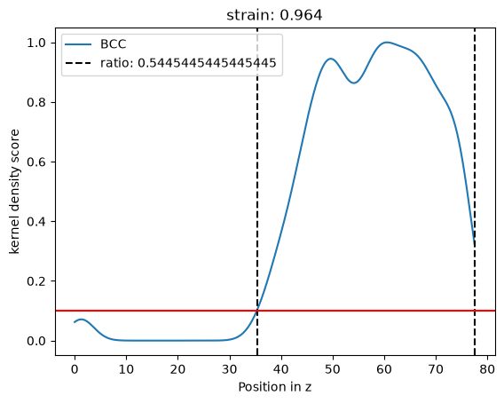
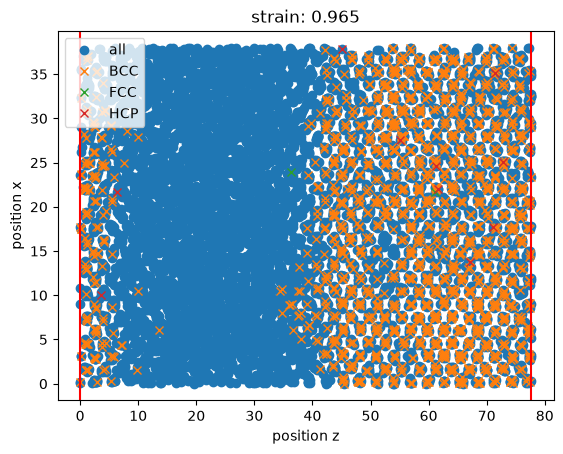
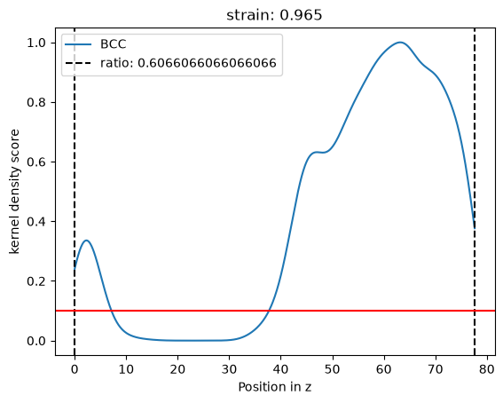
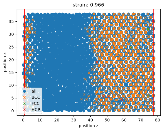
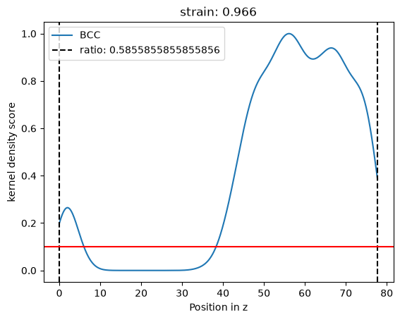
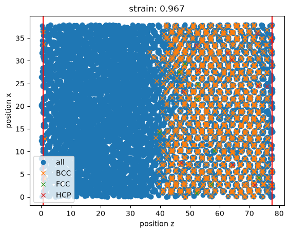
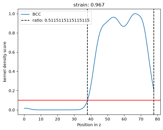
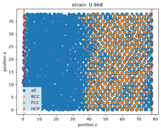
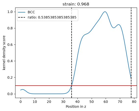
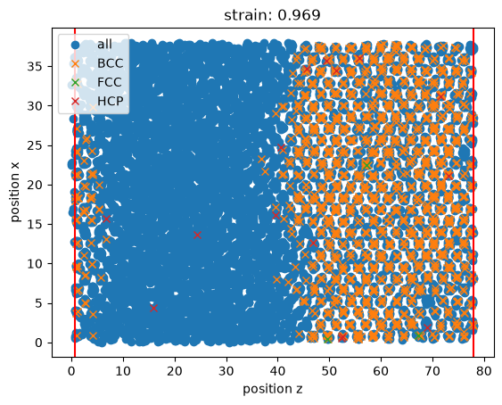
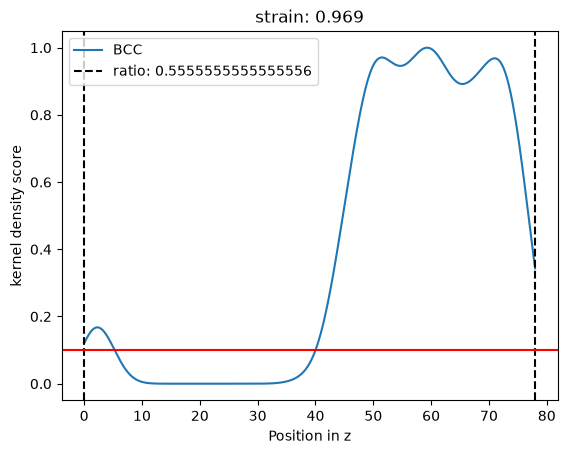
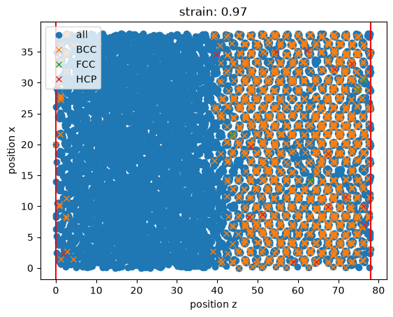
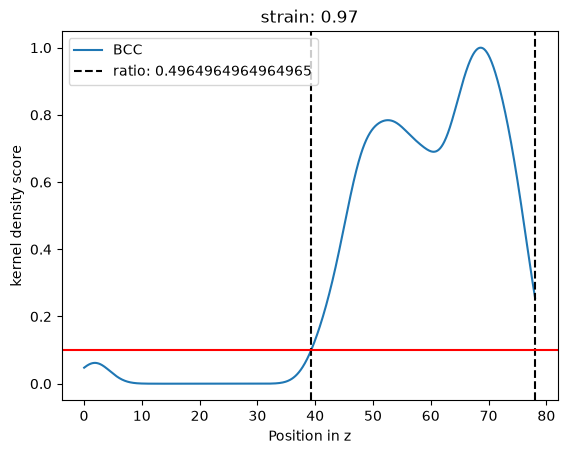
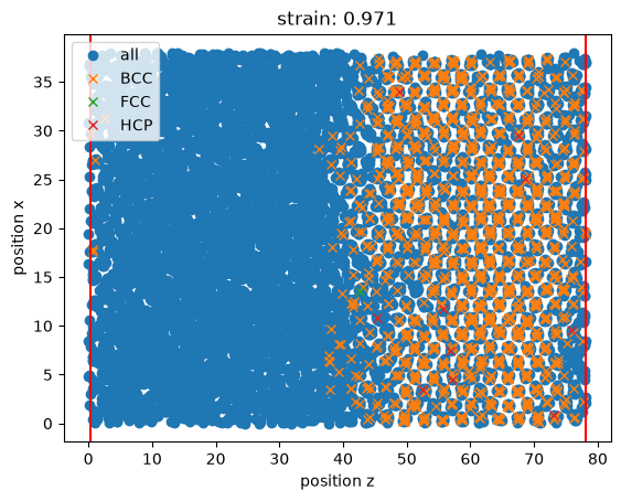
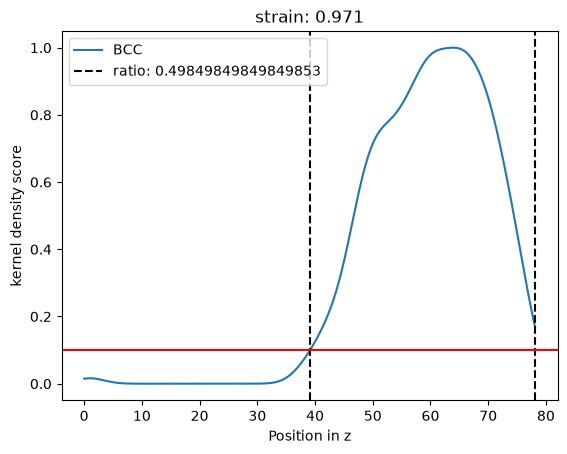
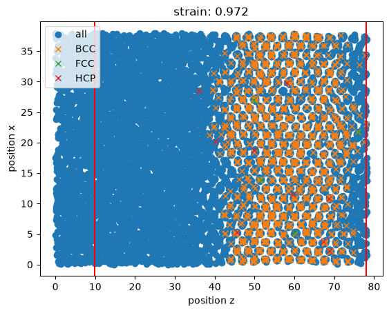
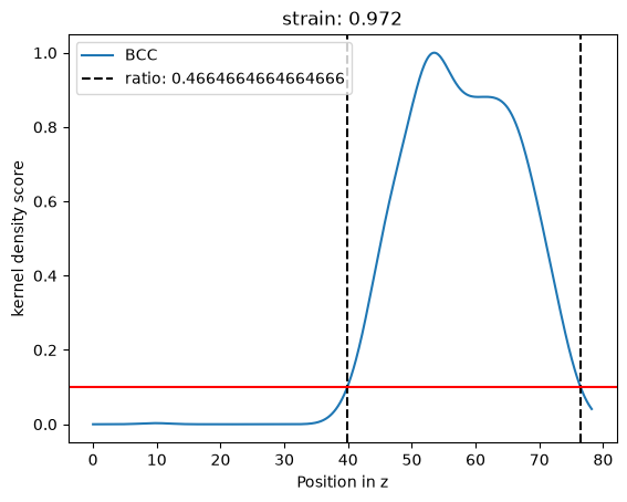
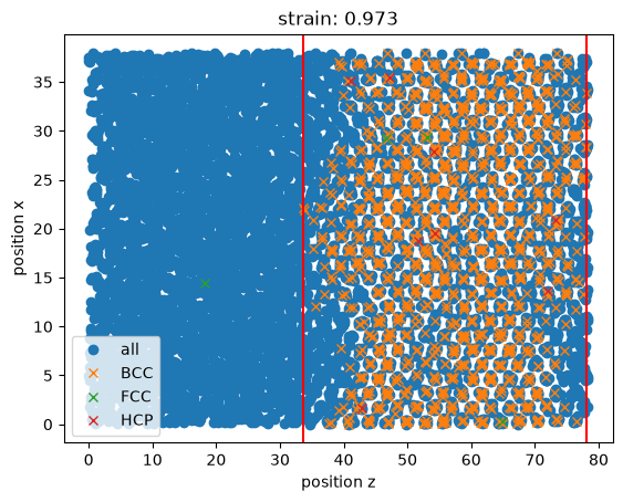
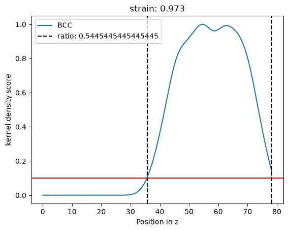
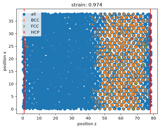
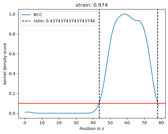
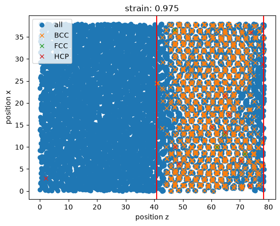
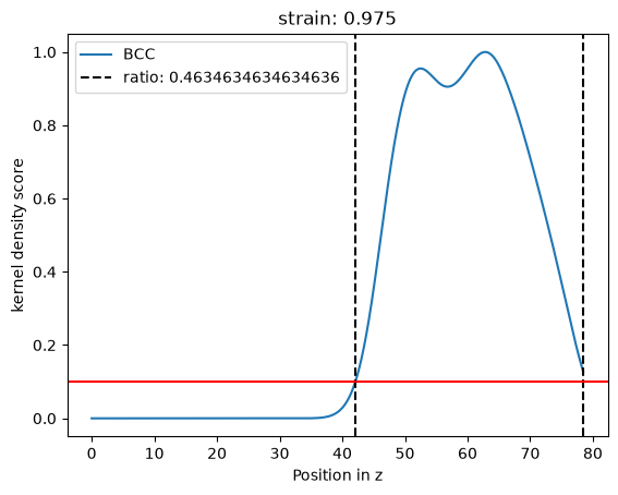
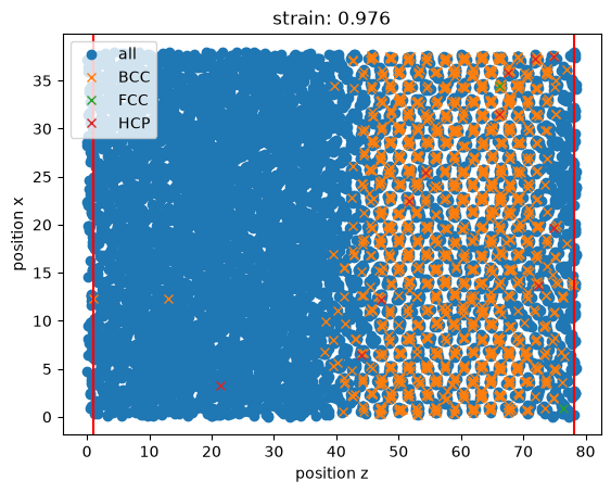
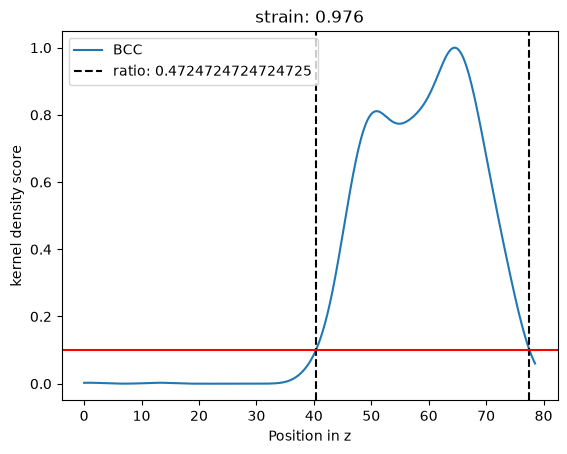
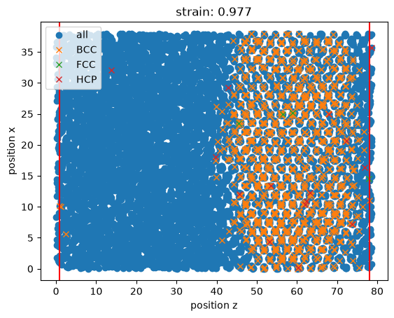
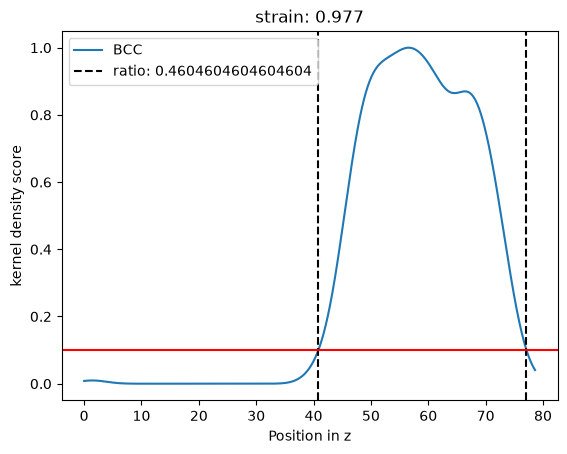
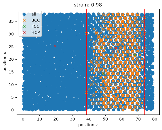
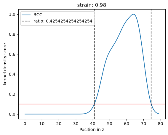
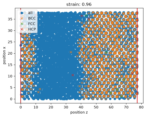
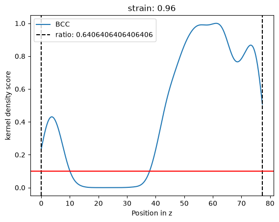
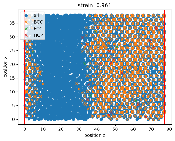
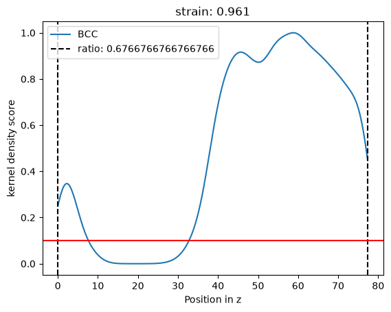
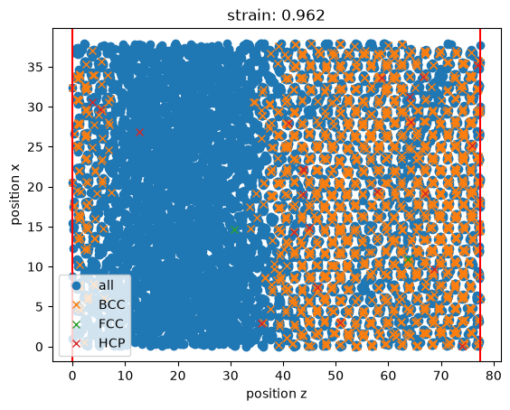
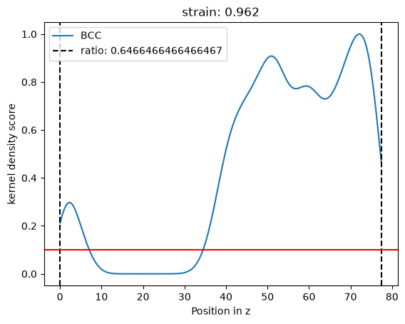
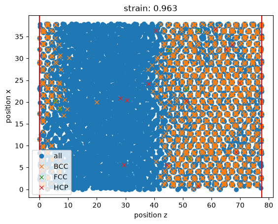
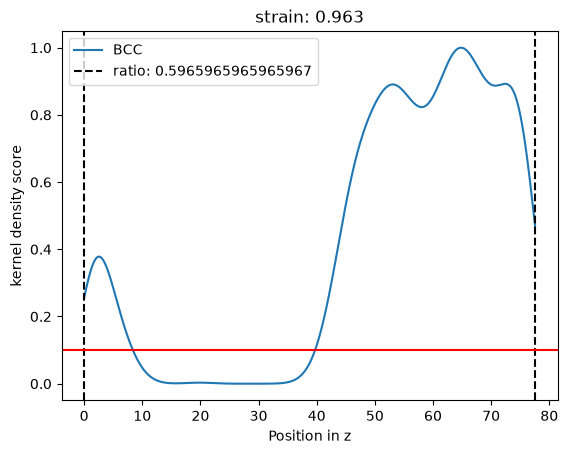
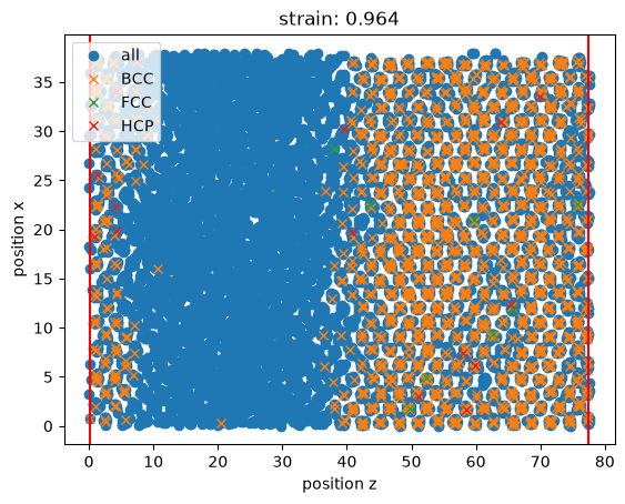
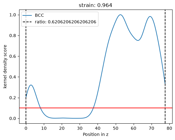
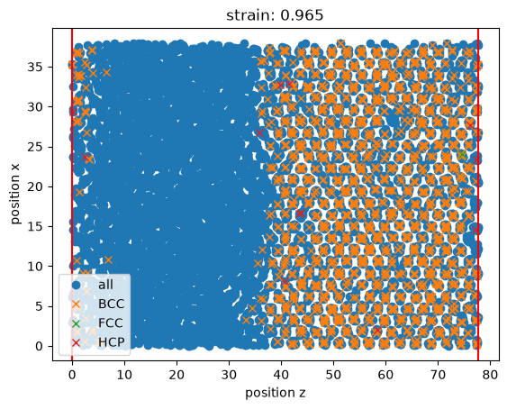
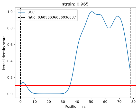
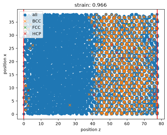
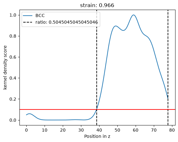
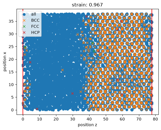
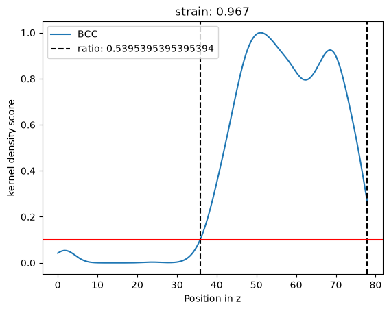
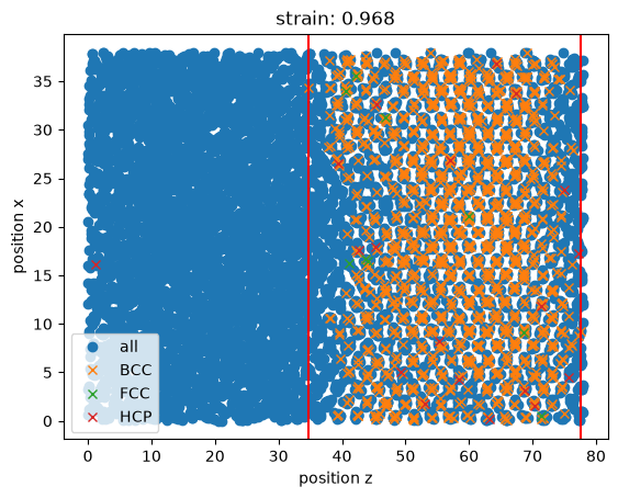
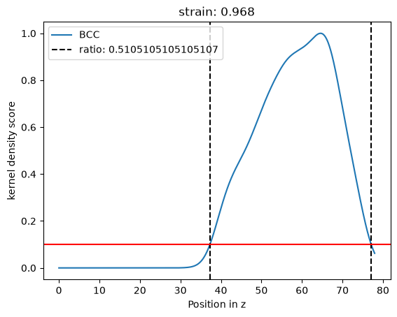
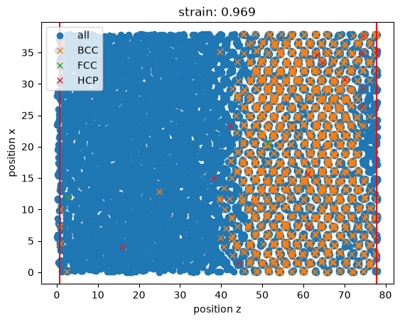
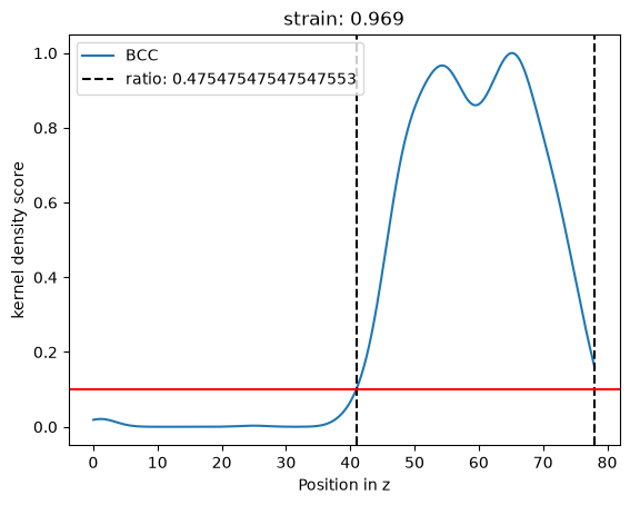
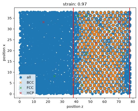
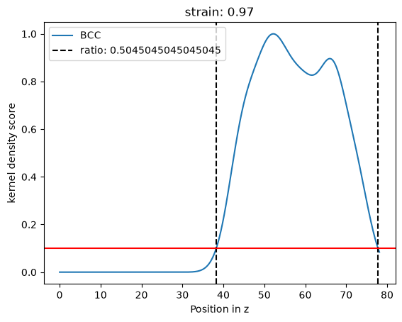
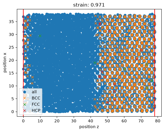
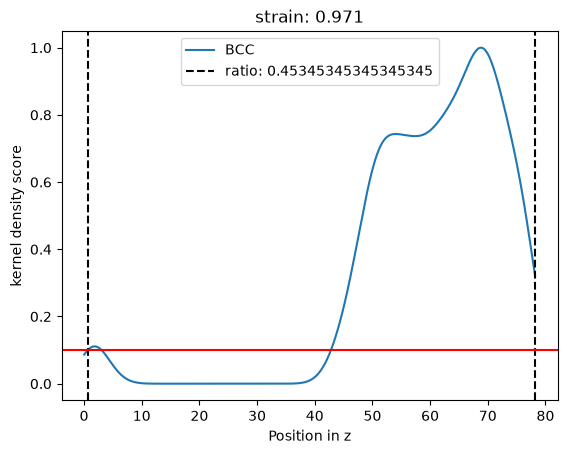
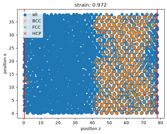
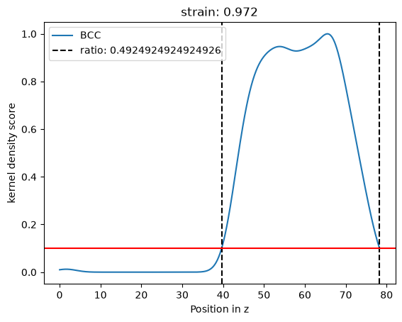
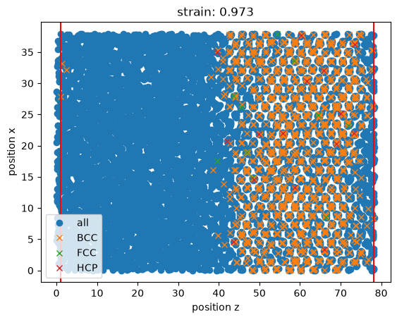
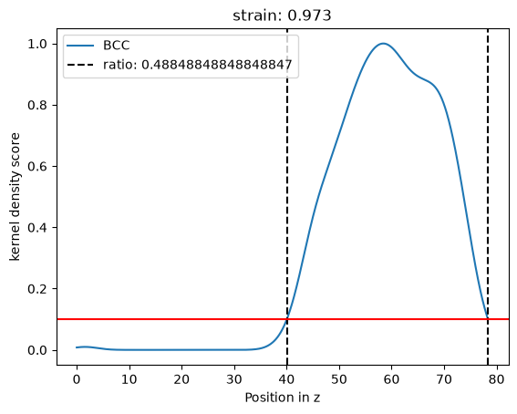
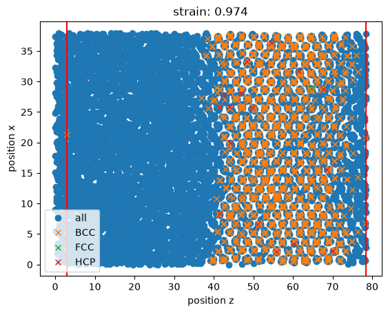
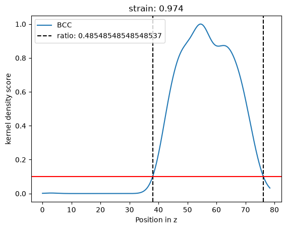
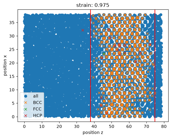
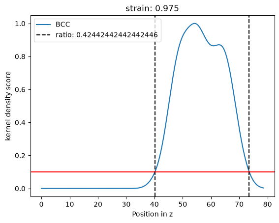
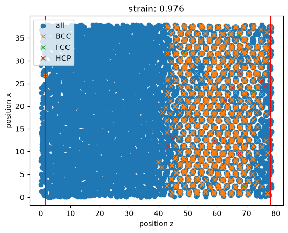
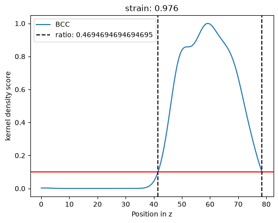
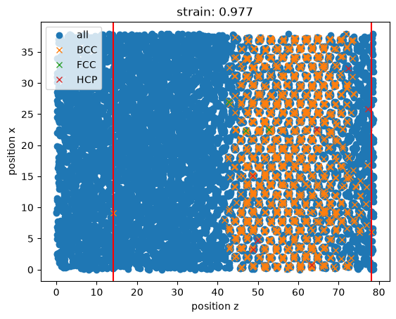
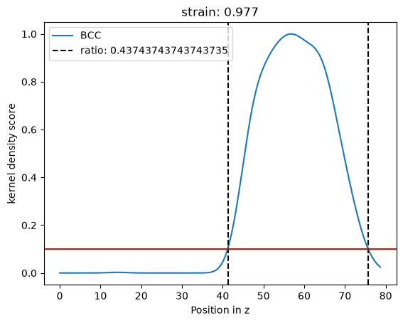
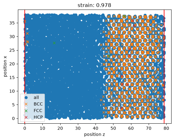
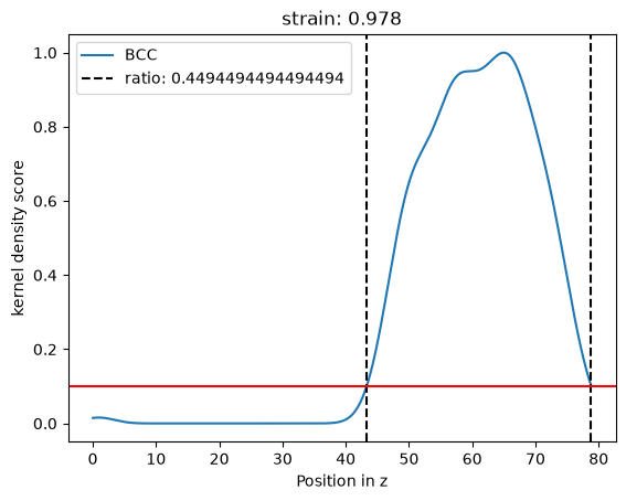
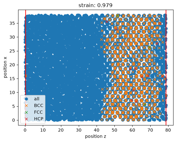
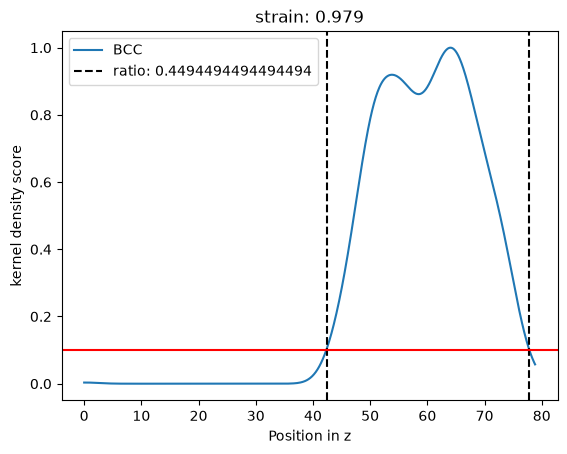
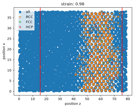
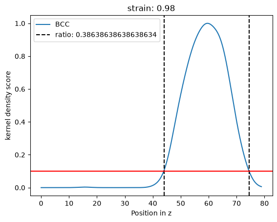
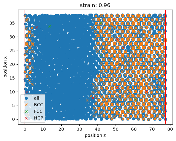
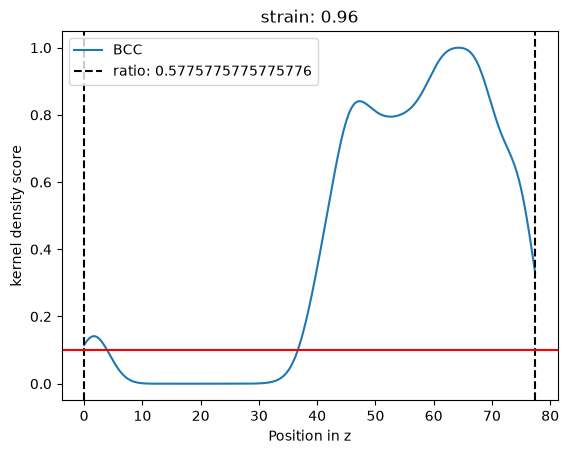
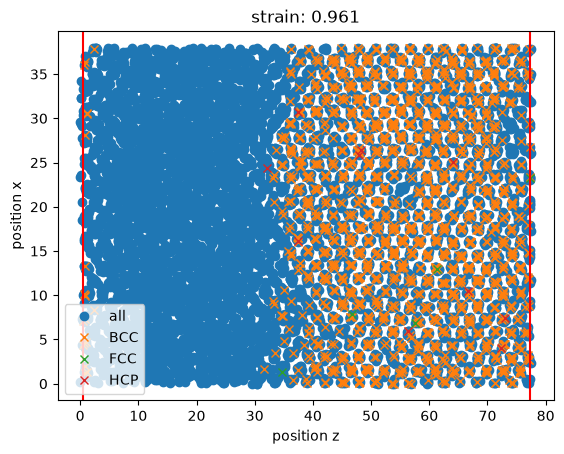
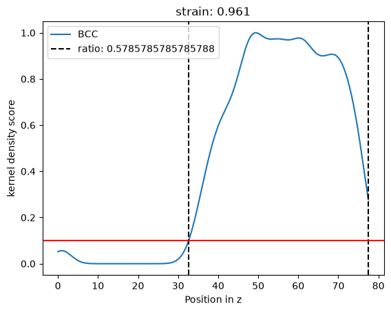
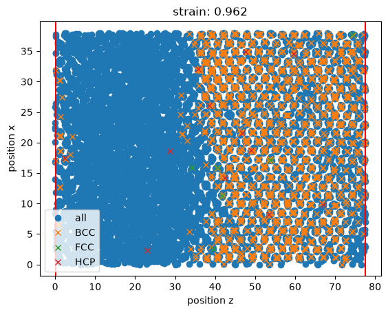
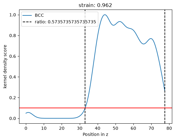
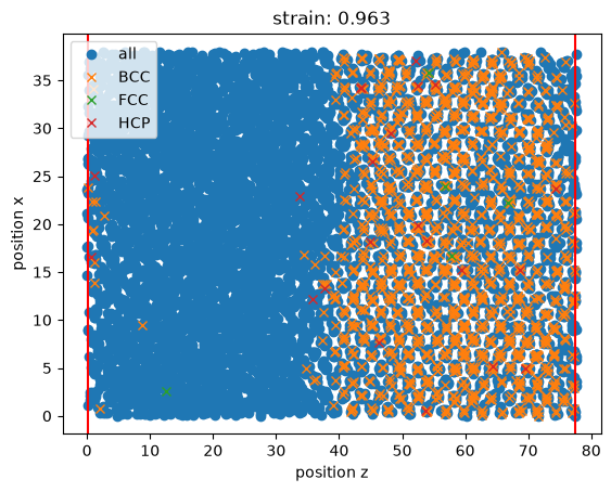
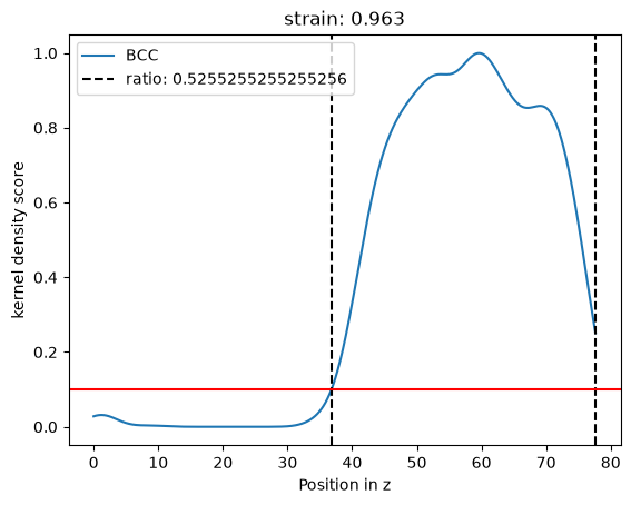
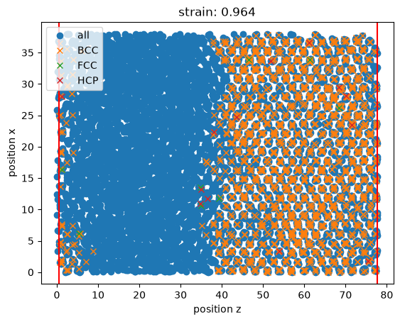
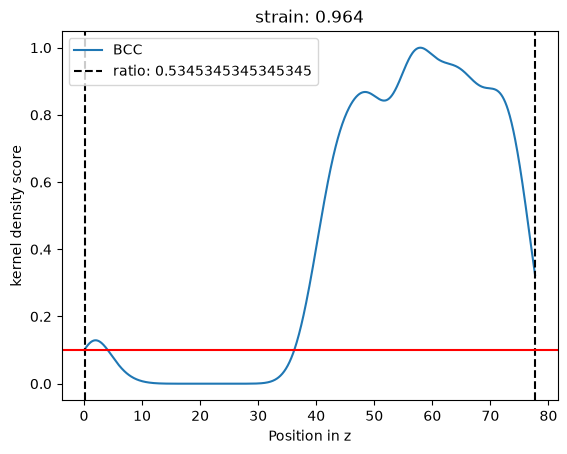
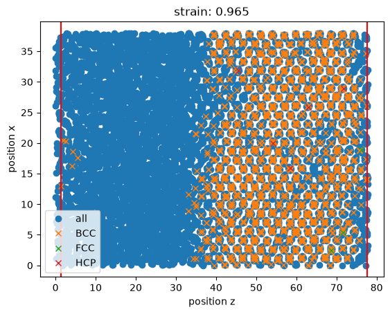
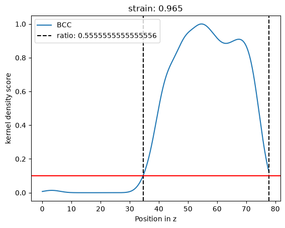
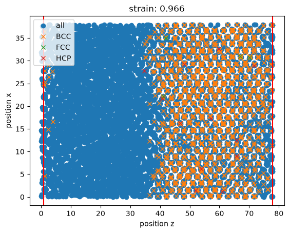
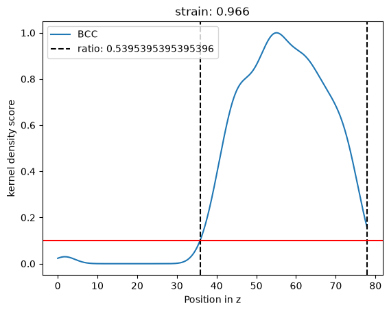
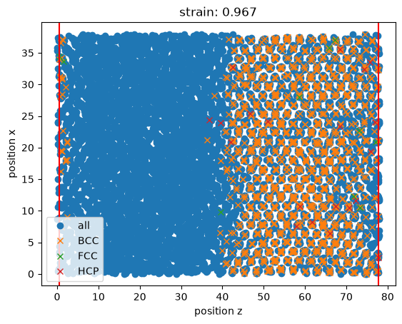
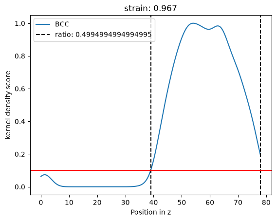
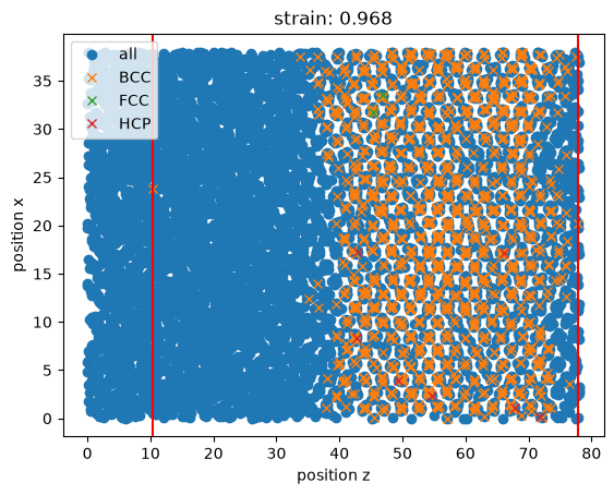
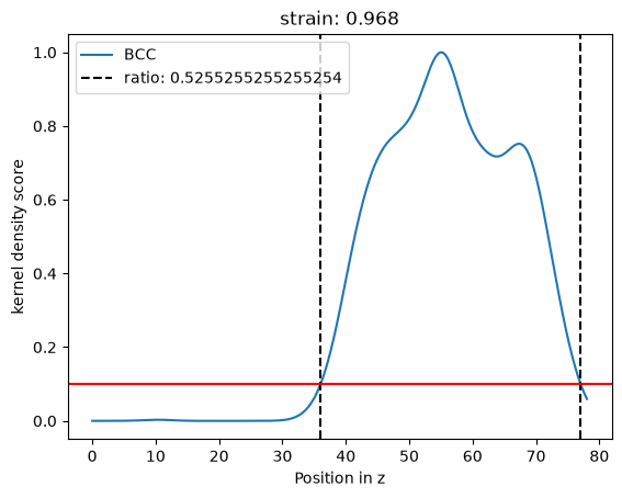
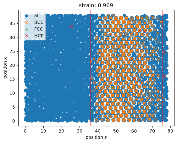
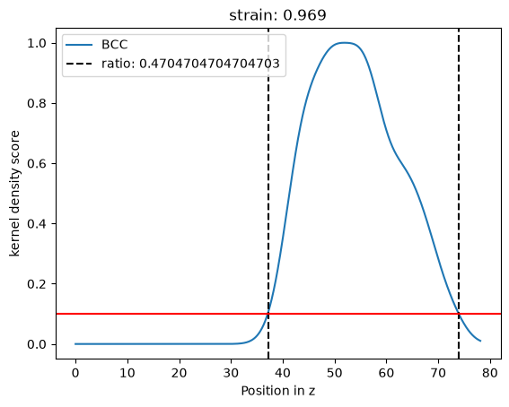
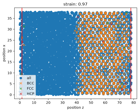
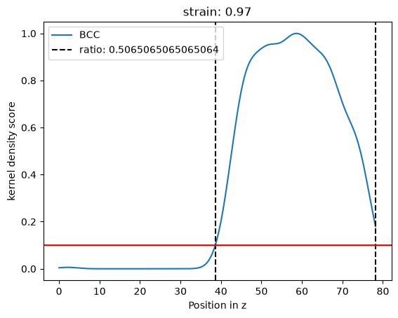
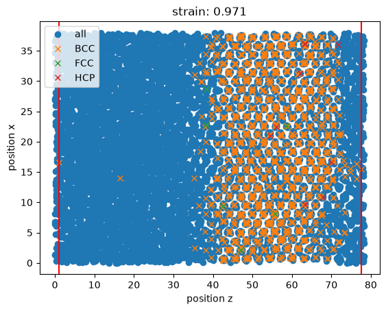
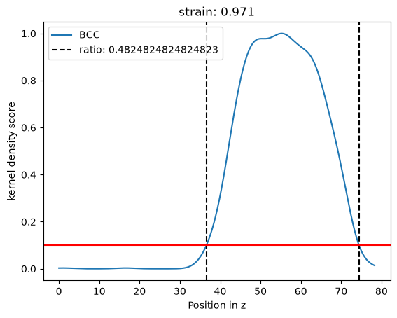
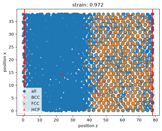
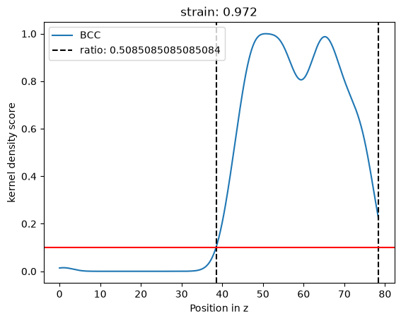
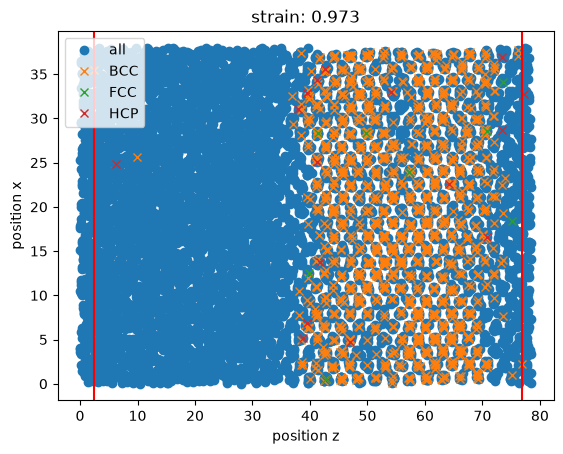
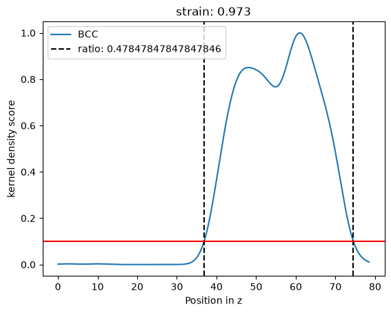
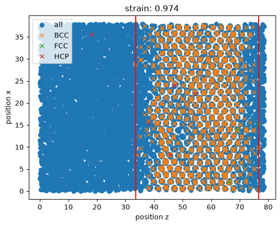
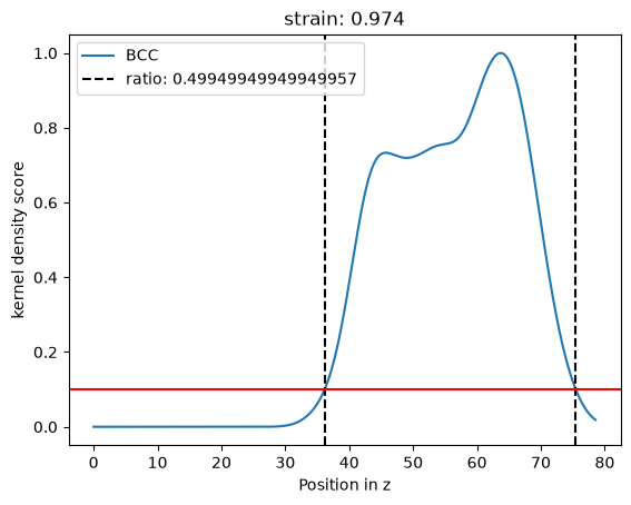
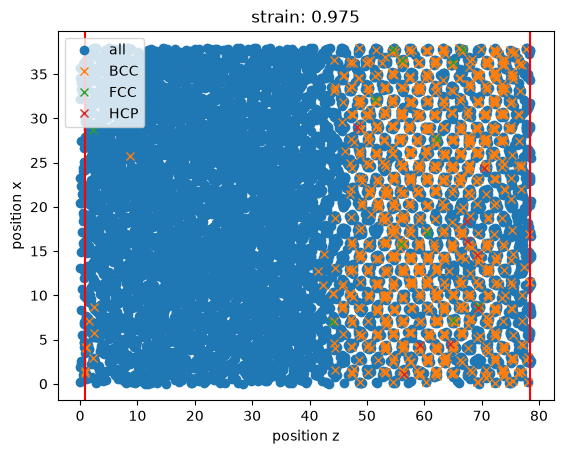
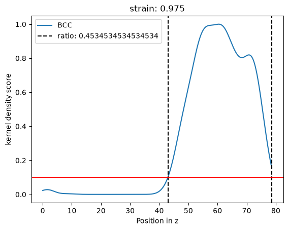
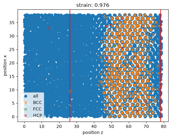
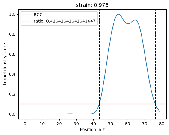
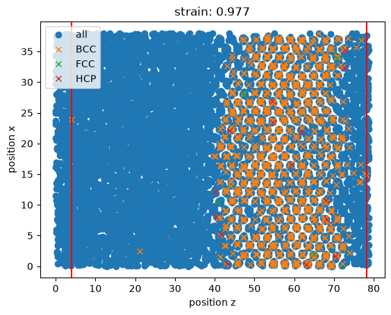
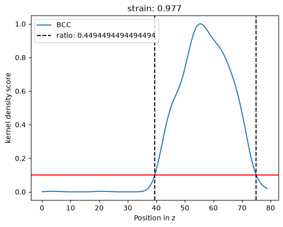
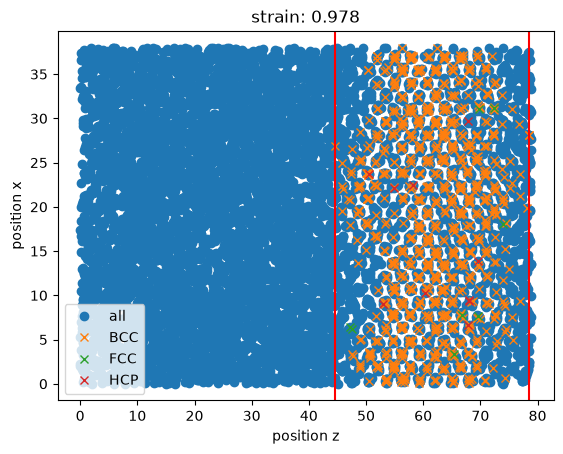
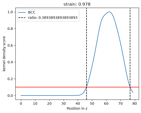
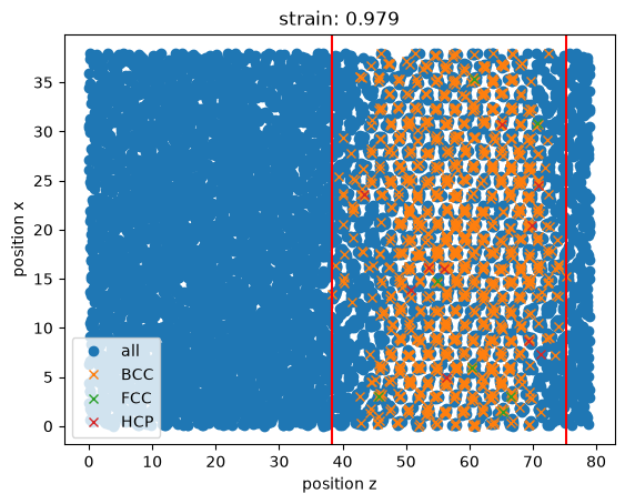
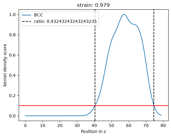
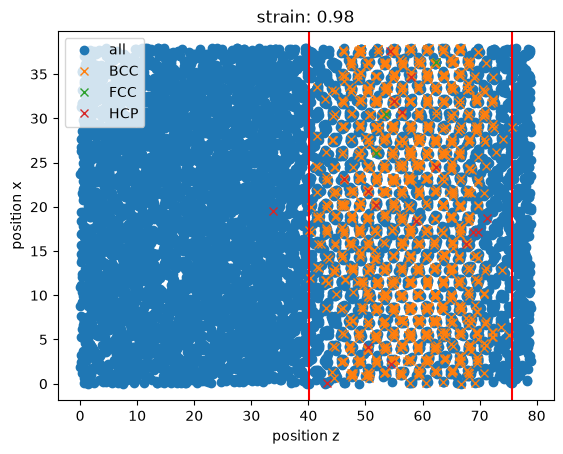
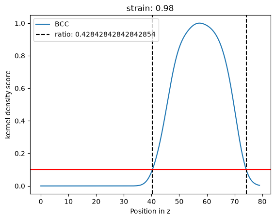
• Structure + CNA scatter plot (one pair of plots per strain) - atom positions in the x-z plane colored by their local CNA classification, with red vertical lines marking the extent of the target crystal structure along z. The second plot of the pair is the kernel-density profile of that classification along z, used to compute the solid/liquid ratio for the strain; the 10% threshold used to locate the phase boundary is shown as a horizontal dashed line.

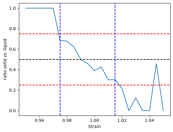
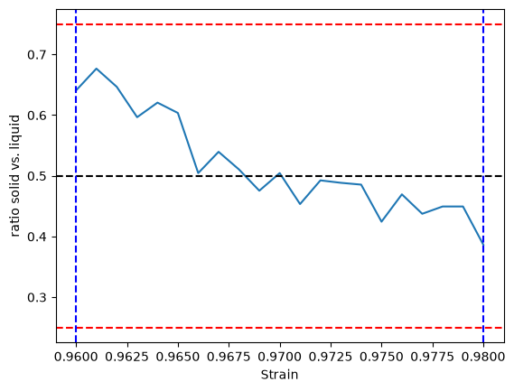
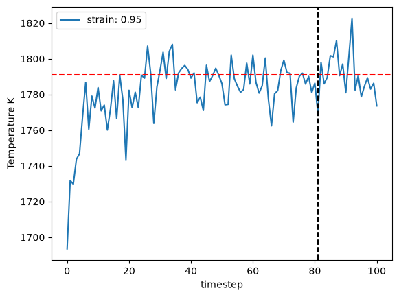
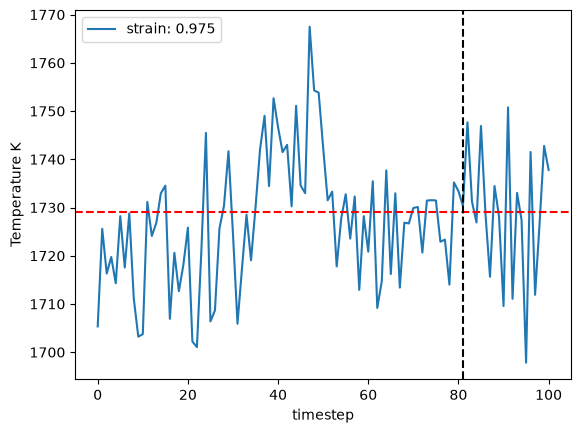
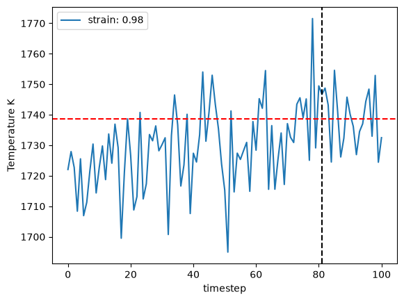
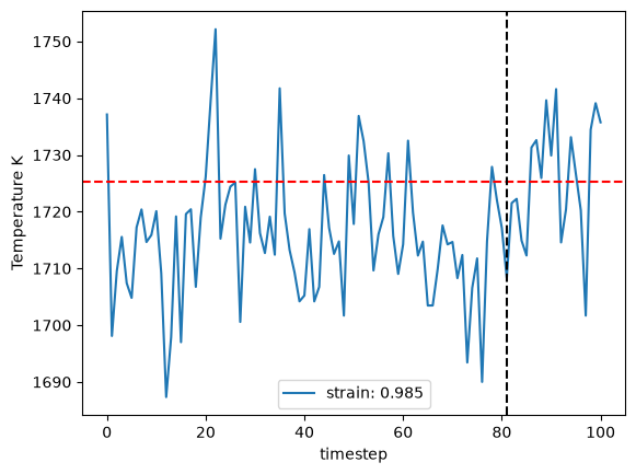
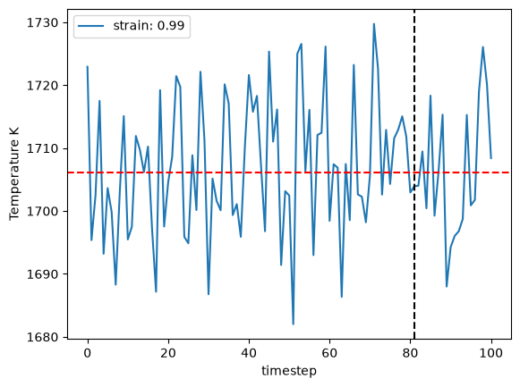
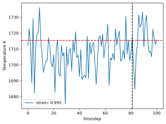
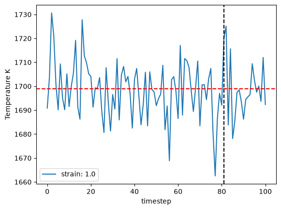
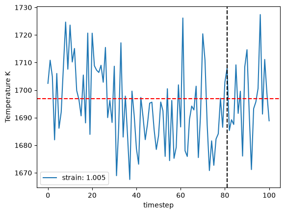
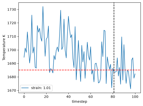
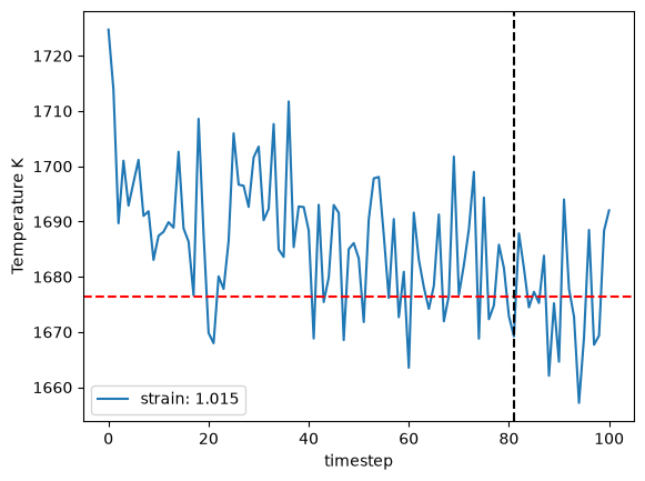
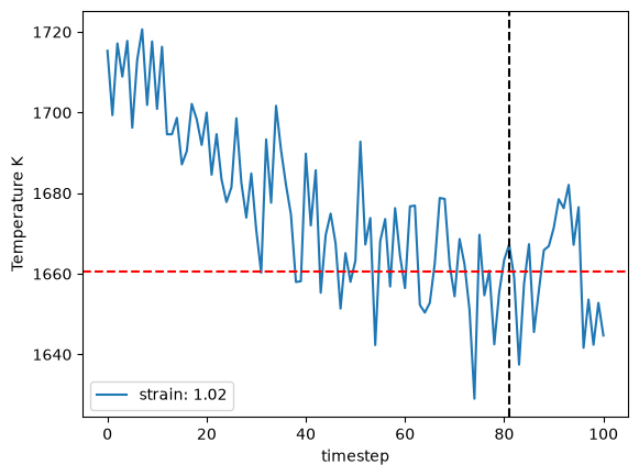
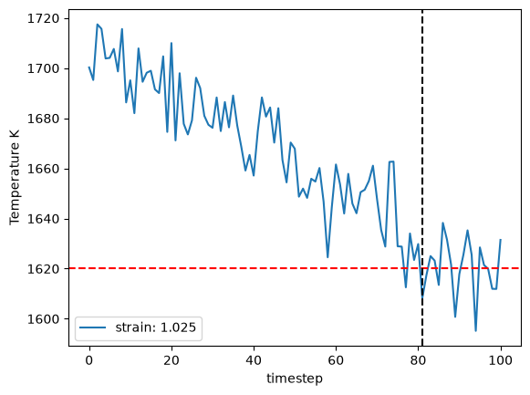
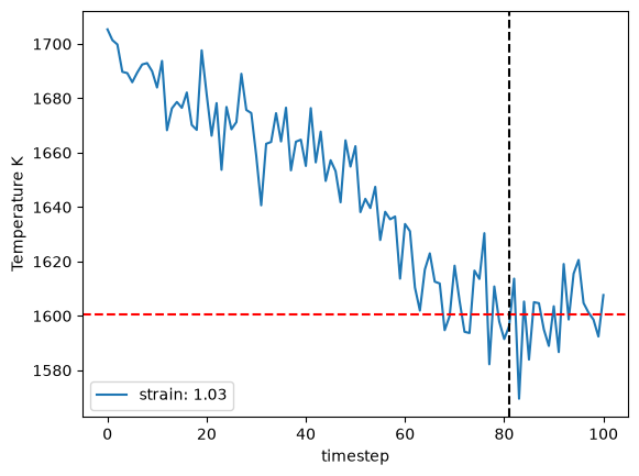
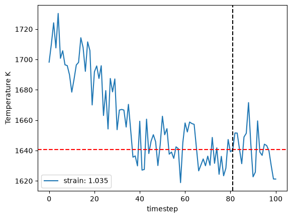
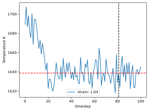
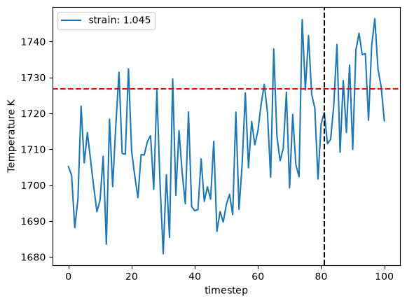
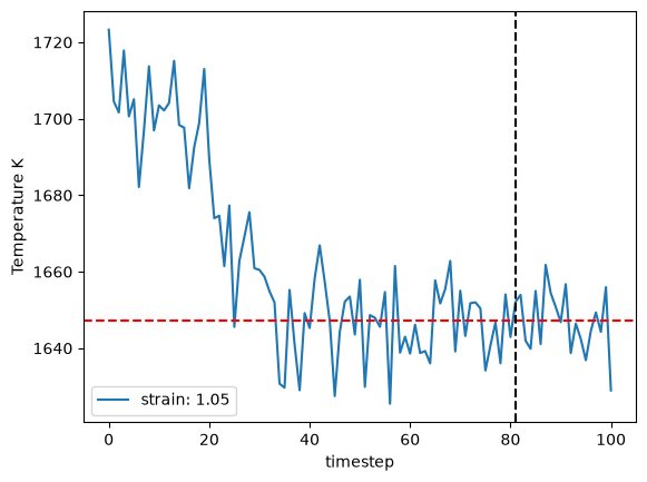
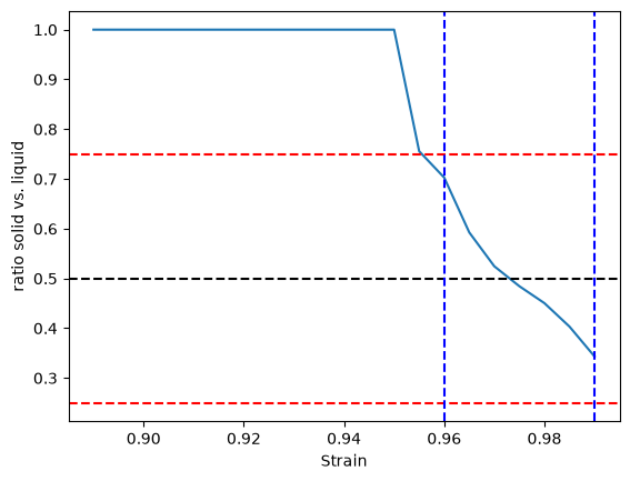
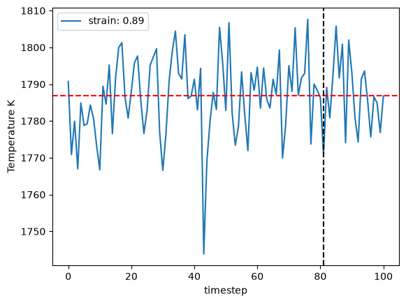
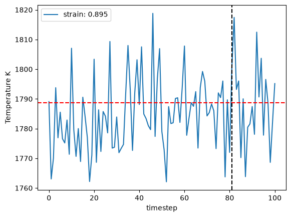
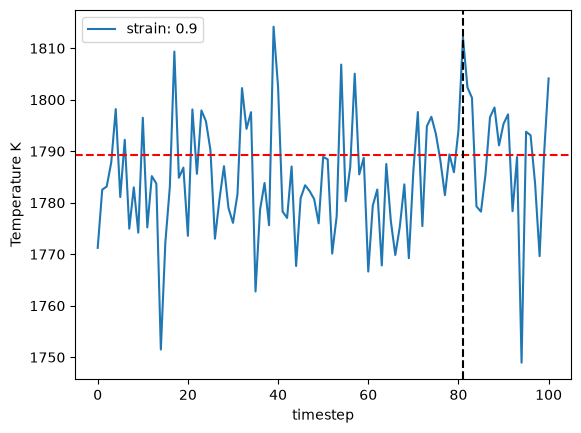
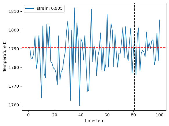
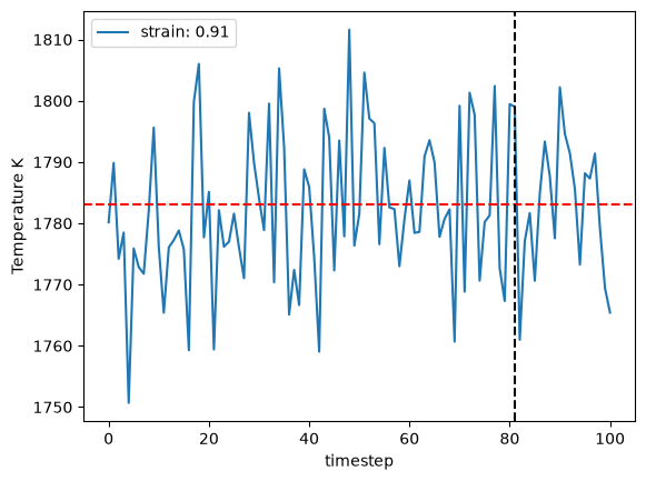
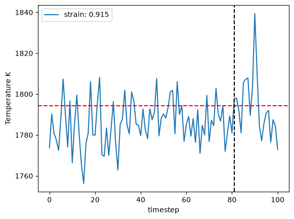
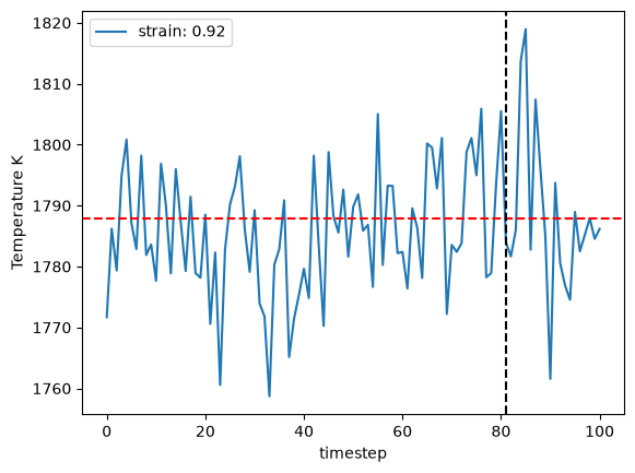
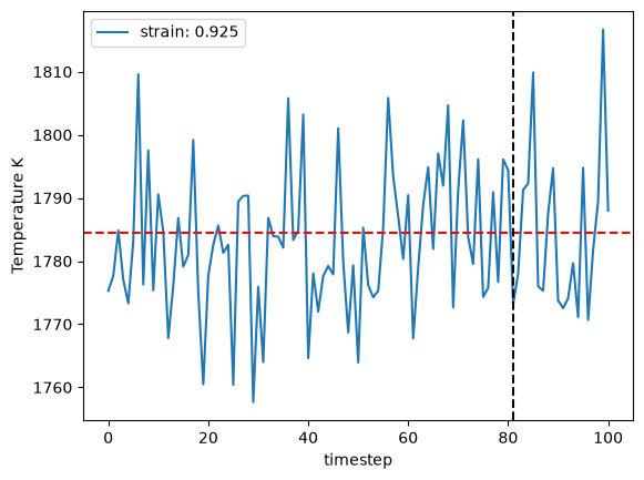
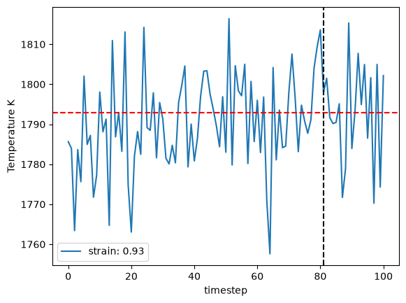
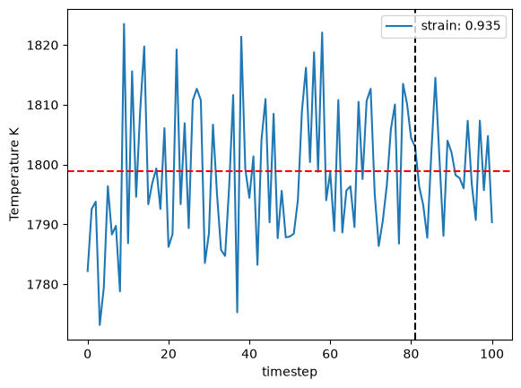
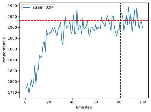
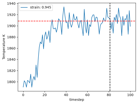
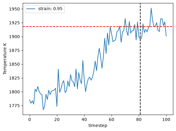
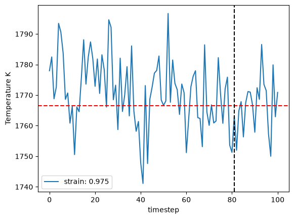
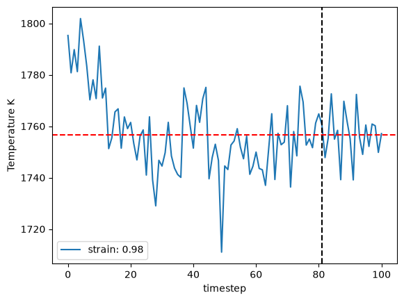
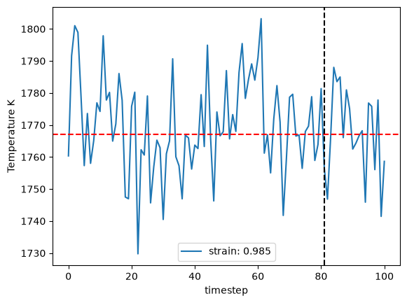
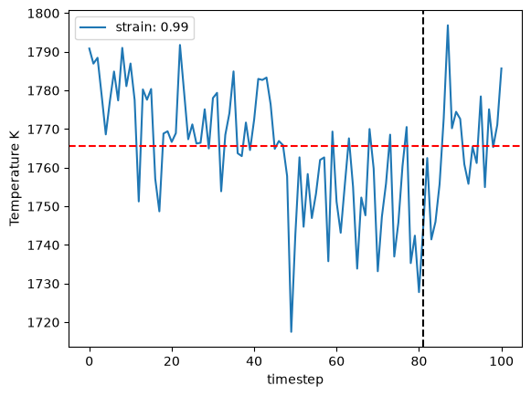
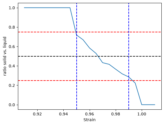
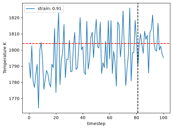
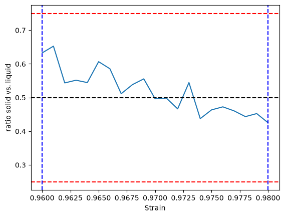
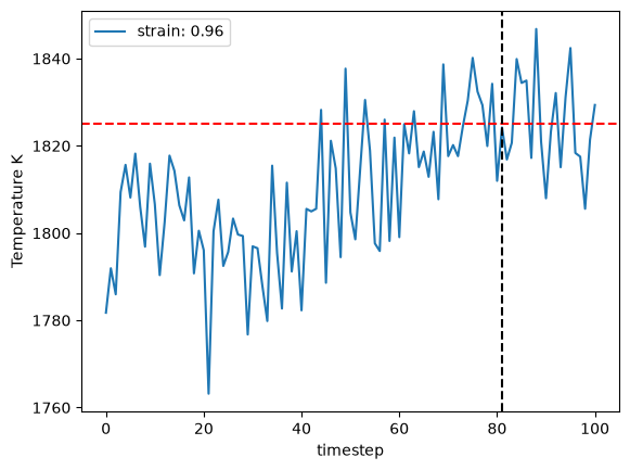
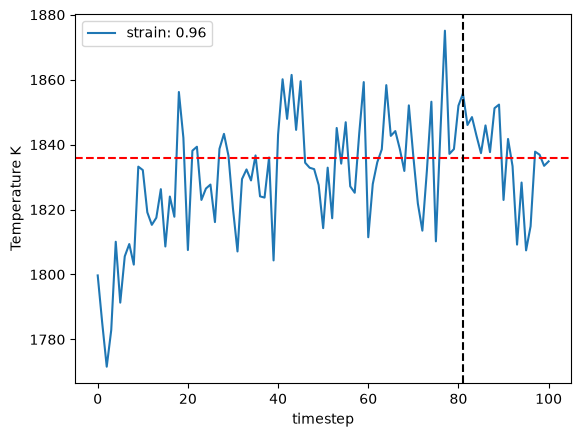
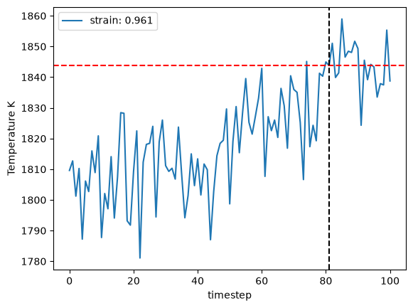
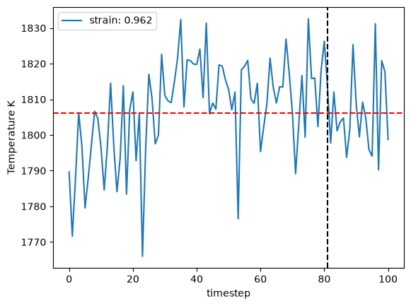
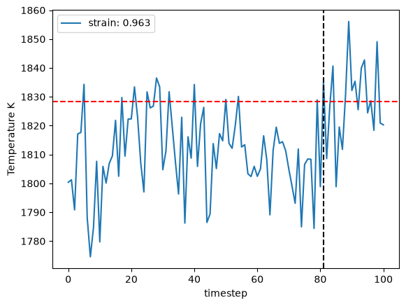
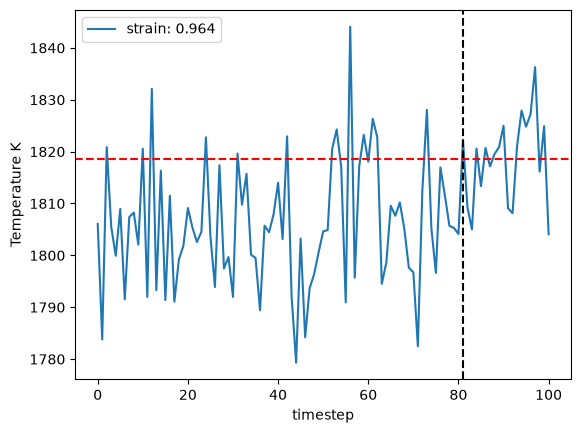
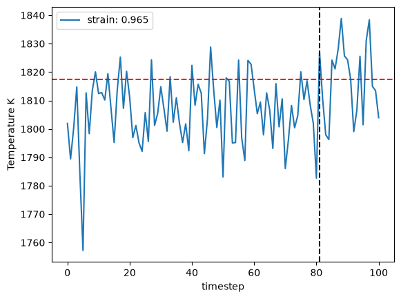
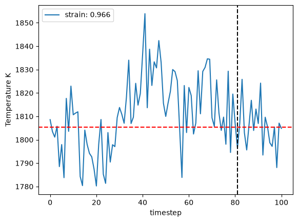
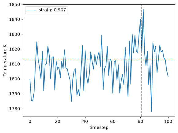
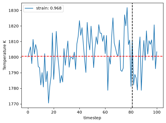
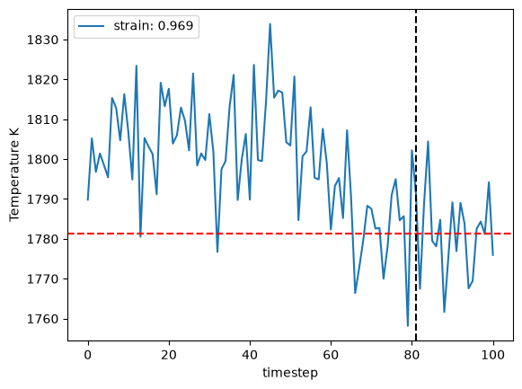
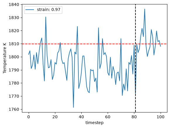
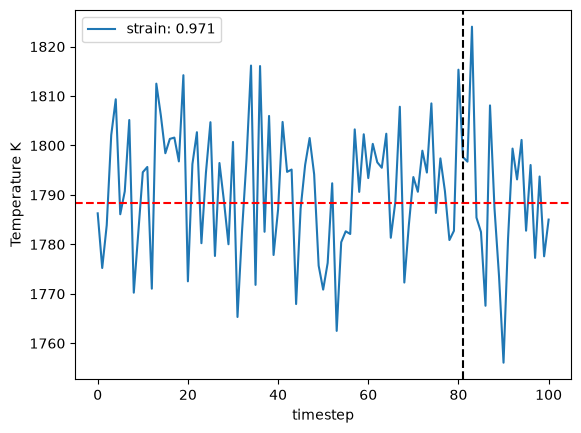
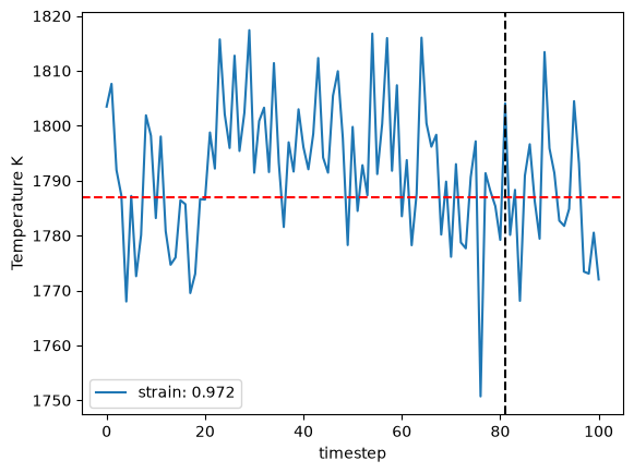
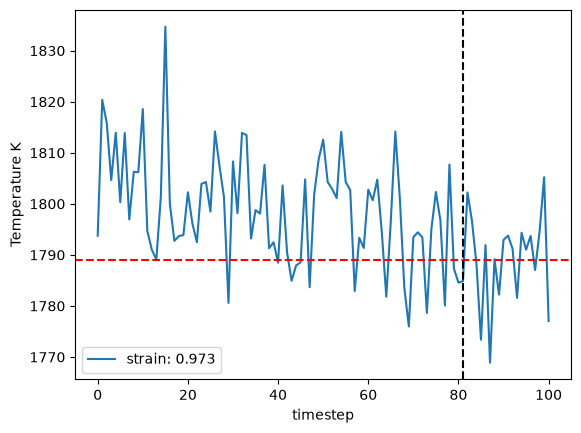
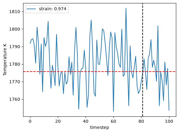
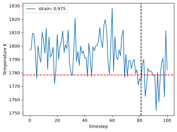
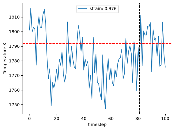
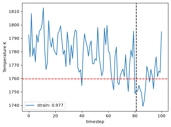
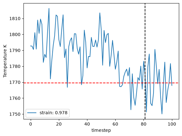
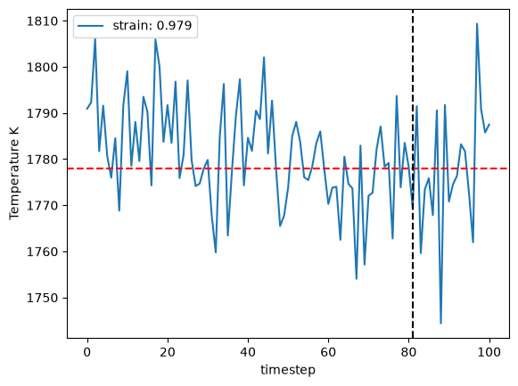
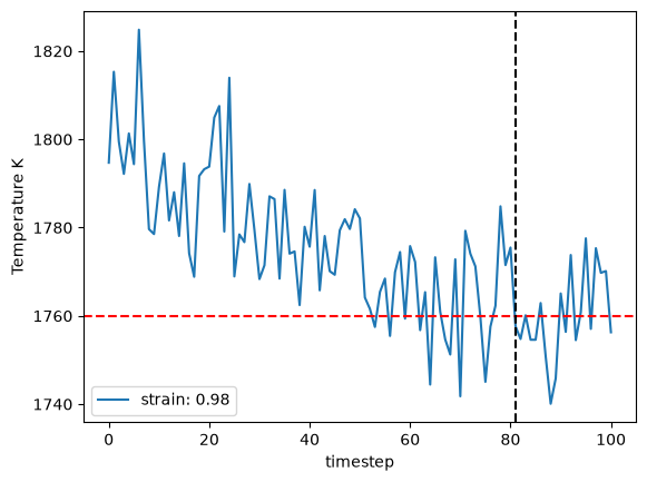
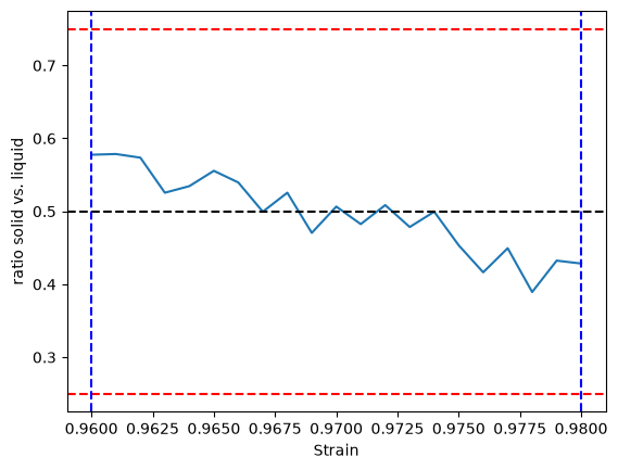
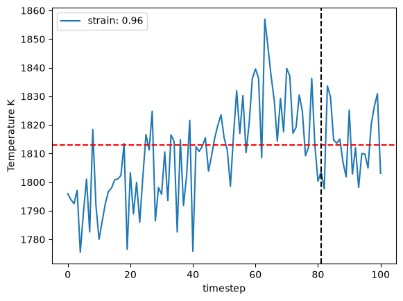
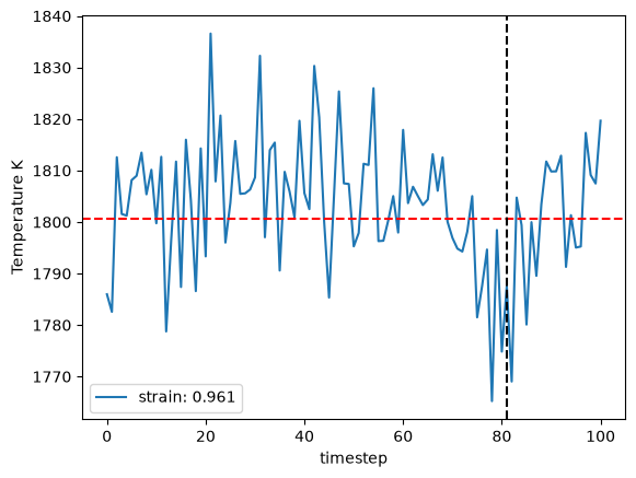
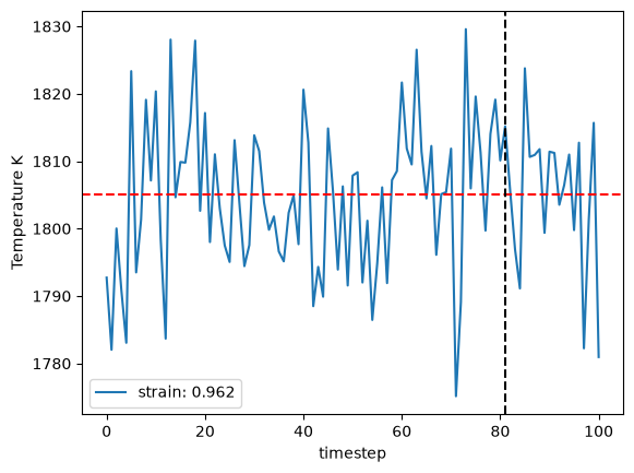
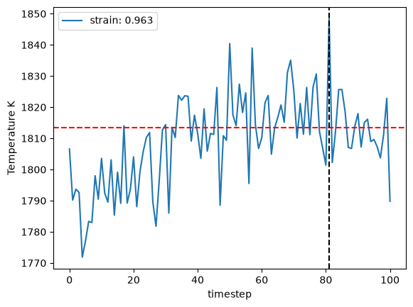
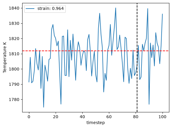
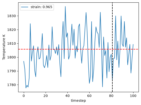
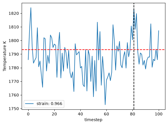
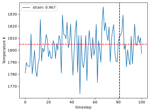
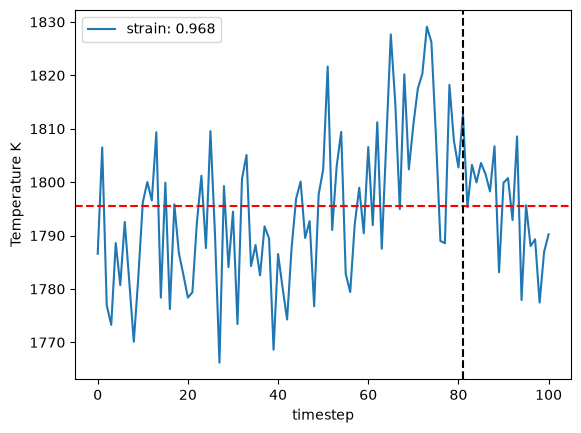
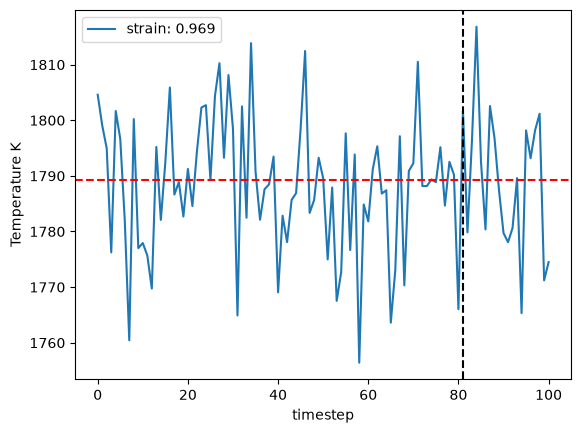
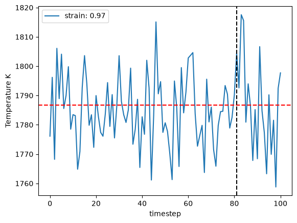
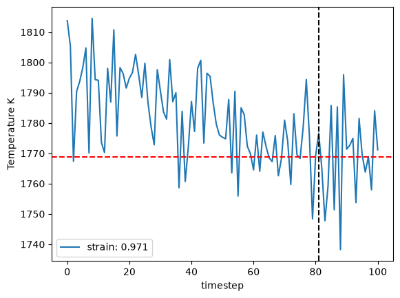
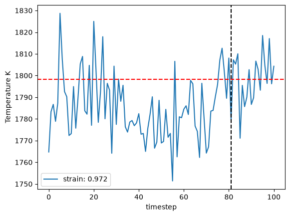
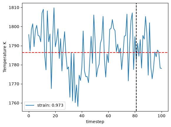
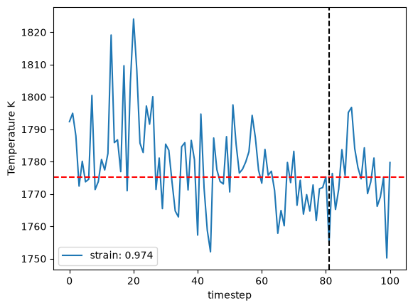
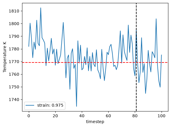
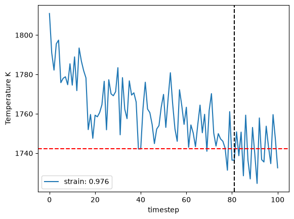
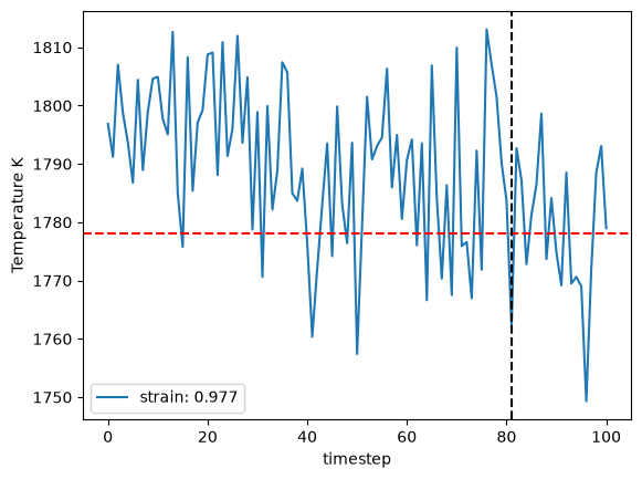
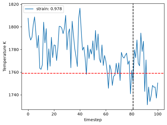
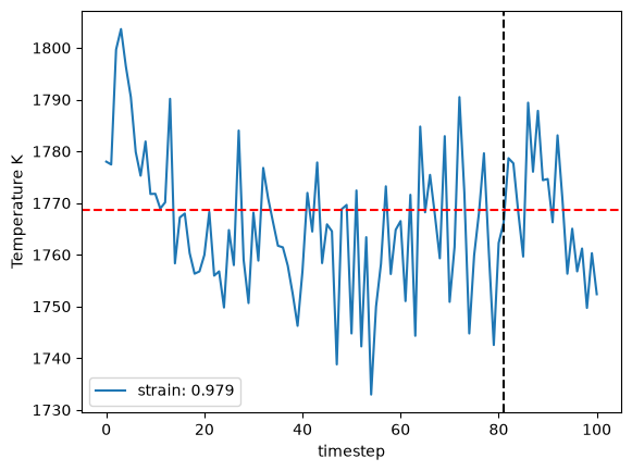
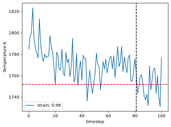
• Ratio vs. strain plot - the solid/liquid ratio of every strain point, with the ±ratio_boundary band around 0.5 (perfect 50/50 coexistence) marked in red and the longest contiguous run of strains inside that band marked with blue dashed lines. Only that run is kept for the fit below; the discarded strains have fully melted or fully solidified and no longer contain a coexisting interface.

• Equilibration plots (one per kept strain) - temperature vs. timestep during the NVE run, with the average of the last 20 steps (dashed red line) used as that strain point’s temperature. Use these to confirm the run reached a stable temperature before it ended.

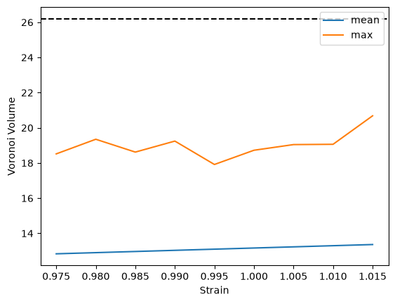
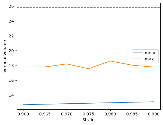
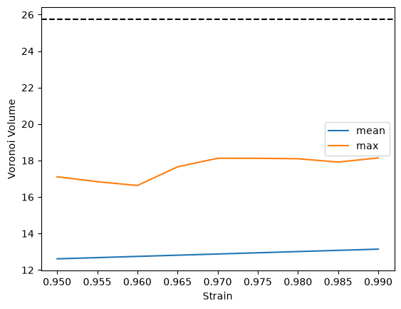
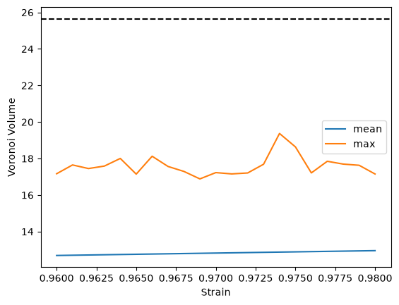
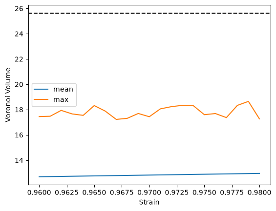
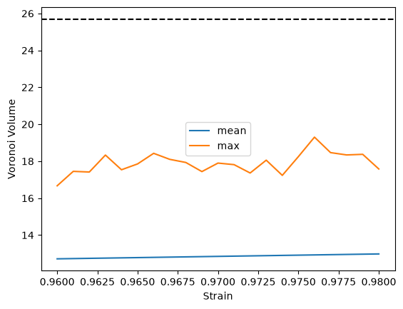
• Voronoi volume plot - mean and maximum Voronoi volume vs. strain; strain points whose maximum exceeds twice the mean (dashed line) have developed an unphysical hole/cavity during the NVE run and are dropped from the fit.

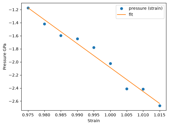
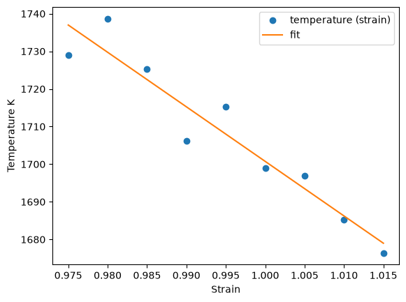
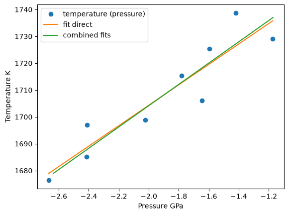
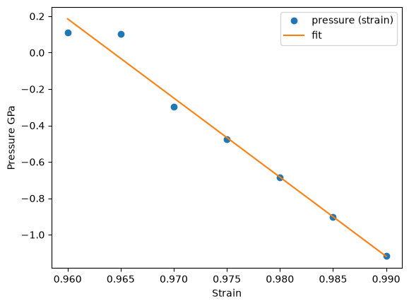
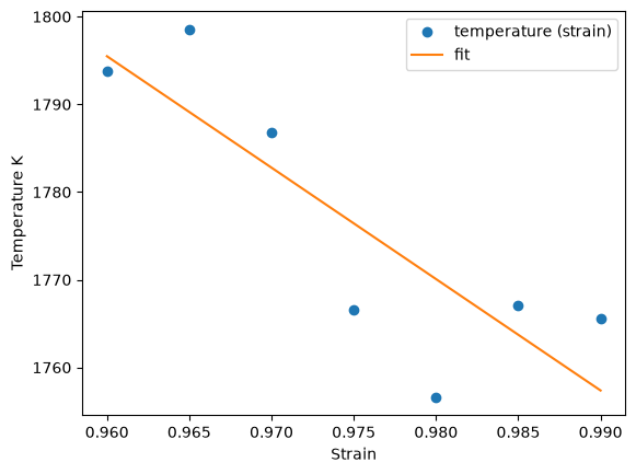
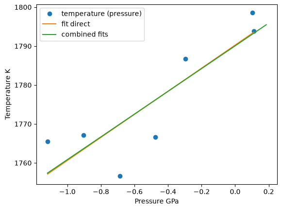
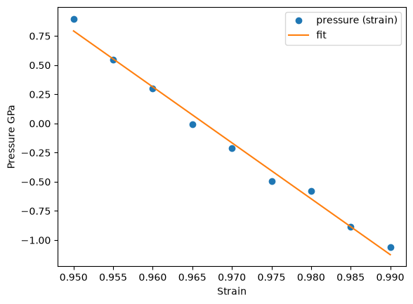
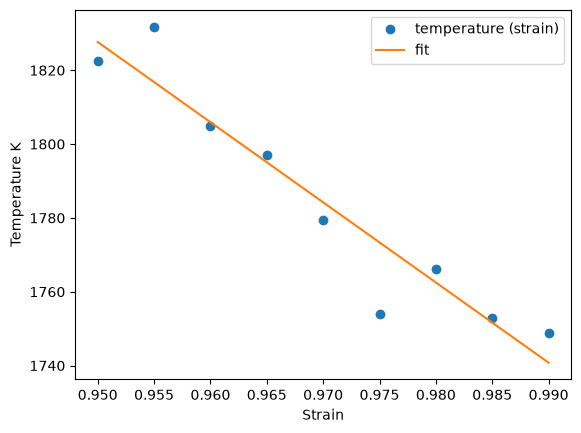
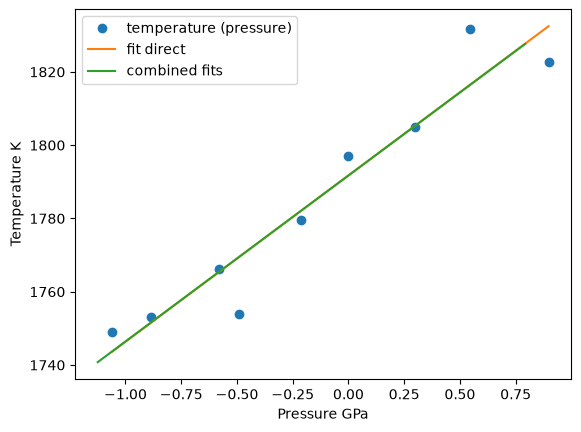
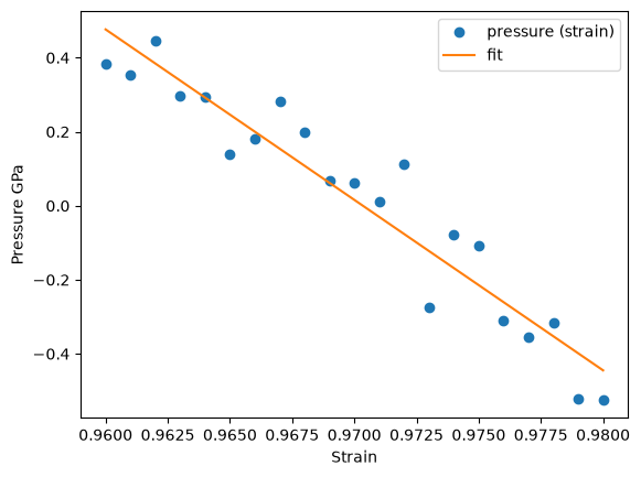
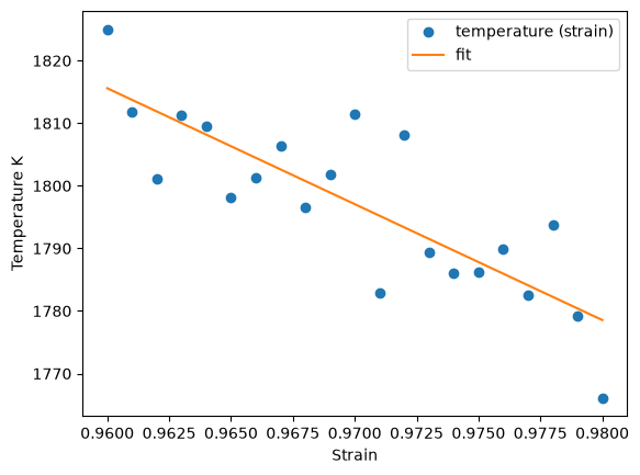
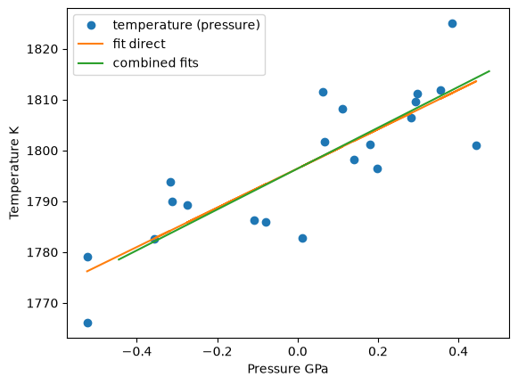
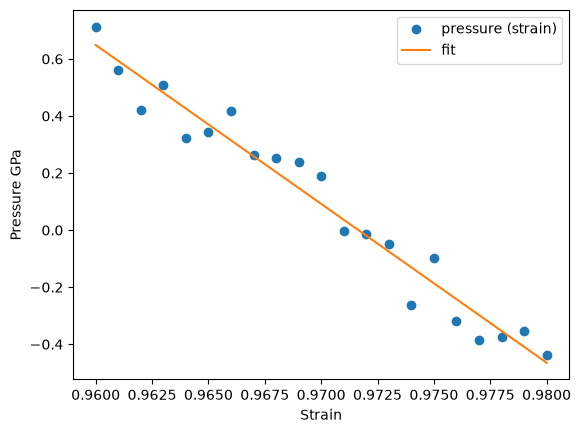
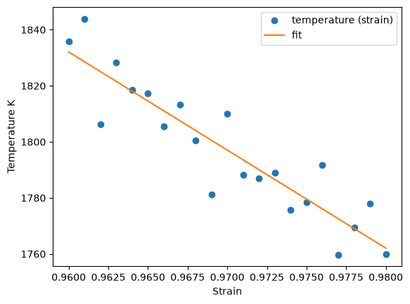
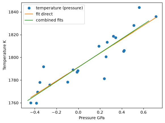
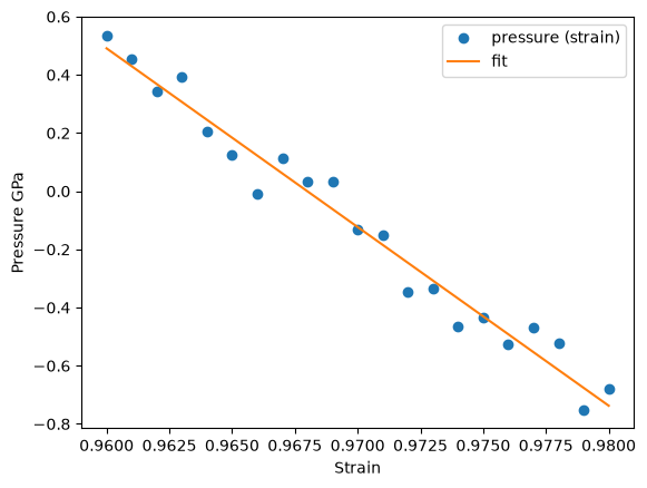
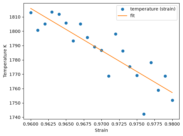
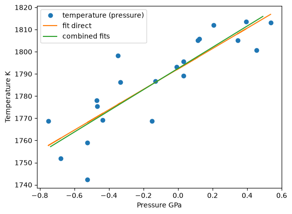
• Pressure/temperature vs. strain, and temperature vs. pressure - linear fits of pressure and temperature against strain, and of temperature against pressure. The temperature at zero pressure (fit_temp_from_press(0.0)) is the melting temperature prediction this iteration produces; it is printed above the plots together with a second estimate obtained by combining the two strain-based fits, as a consistency check between the two ways of extrapolating to zero pressure.

Pass debug_plot=False to run_interface_iteration() to suppress all of the above, e.g. for unattended runs on a cluster.

temperature_next = round_temperature_next(temperature_next)
temperature_next

np.int64(1711)

def run_interface_iteration(
    basis,
    temperature_next,
    project_parameter,
    project_path,
    timestep,
    nve_run_time_steps,
    fit_range,
    center,
    lmp_command,
    max_workers=4,
    debug_plot=True,
):
    """
    Run one iteration of the solid-liquid interface method and predict the next melting
    temperature estimate:

    1. equilibrate the solid at the target temperature (NPT)
    2. partially melt one half of the cell and re-equilibrate to build a solid-liquid interface (NPT)
    3. scan a series of strains around the current lattice parameter (NVT + NVE)
    4. classify each strain point as solid- or liquid-dominated and keep the coexistence region
    5. fit pressure and temperature vs. strain to predict the next melting temperature estimate
    """
    temperature_next = round_temperature_next(temperature_next)

    with SingleNodeExecutor(cache_directory="cache", max_workers=max_workers) as exe:

        # Step 2a: equilibrate the solid at the target temperature (NPT)
        structure_npt_solid = exe.submit(
            npt_solid,
            lmp_command=lmp_command,
            temperature=temperature_next,
            basis=basis,
            project_parameter=project_parameter,
            project_path=project_path,
            timestep=timestep,
        ).result()
        structure_npt_solid.set_velocities(np.zeros_like(structure_npt_solid.get_velocities()))

        # Step 2b: partially melt one half and re-equilibrate to build a solid-liquid interface (NPT)
        structure_npt_liquid_low = exe.submit(
            npt_liquid,
            lmp_command=lmp_command,
            temperature_solid=temperature_next,
            temperature_liquid=temperature_next + 1000,
            basis=structure_npt_solid,
            project_parameter=project_parameter,
            project_path=project_path,
            timestep=timestep,
        ).result()
        basis_relative = remove_selective_dynamics(structure_npt_liquid_low)

        # Step 2c: scan a series of strains around the current lattice parameter (NVT + NVE).
        # Every strain point is independent of every other -- this is the parallelization point of
        # the workflow. See the note below on replacing this `for` loop with a parallel executor.
        strain_lst = get_strain_lst(
            fit_range=fit_range, points=project_parameter["points"], center=center,
        )
        strain_futures = []
        for strain in strain_lst:
            strain_futures.append(
                exe.submit(
                    run_strain_point,
                    strain=strain,
                    lmp_command=lmp_command,
                    basis_relative=basis_relative,
                    temperature_next=temperature_next,
                    nve_run_time_steps=nve_run_time_steps,
                    project_parameter=project_parameter,
                    project_path=project_path,
                    timestep=timestep,
                )
            )

        strain_results = [future.result() for future in strain_futures]

    # Step 2d: classify each strain point as solid- or liquid-dominated
    ratio_lst = plot_solid_liquid_ratio(
        strain_results=strain_results,
        project_parameter=project_parameter,
        debug_plot=debug_plot,
    )
    selected_results, sl_flag = ratio_selection(
        strain_results=strain_results,
        ratio_lst=ratio_lst,
        ratio_boundary=project_parameter["ratio_boundary"],
        debug_plot=debug_plot,
    )

    # Step 2e: fit pressure and temperature vs. strain to predict the next melting temperature
    if len(selected_results) > 2:
        plot_equilibration(strain_results=strain_results, debug_plot=debug_plot)
        ind = check_for_holes(strain_results=selected_results)
        selected_results = [r for r, keep in zip(selected_results, ind) if keep]
        (
            temperature_next,
            temperature_mean,
            temperature_left,
            temperature_right,
        ) = plot_melting_point_prediction(
            strain_results=selected_results,
            boundary_value=project_parameter["boundary_value"],
            debug_plot=True,
        )
    elif sl_flag < 0:
        temperature_next, temperature_mean, temperature_left, temperature_right = (
            temperature_next * 0.90, 0.0, 0.0, 0.0,
        )
    else:
        temperature_next, temperature_mean, temperature_left, temperature_right = (
            temperature_next * 1.10, 0.0, 0.0, 0.0,
        )

    strain_result_lst = [r.strain for r in selected_results]
    pressure_result_lst = [r.pressure for r in selected_results]
    return (
        temperature_next,
        temperature_mean,
        temperature_left,
        temperature_right,
        strain_result_lst,
        pressure_result_lst,
    )

temperature_next, temperature_mean, temperature_left, temperature_right, strain_result_lst, pressure_result_lst = run_interface_iteration(
    basis=basis_minimize_vol.repeat([1,1,2]),
    temperature_next=temperature_next,
    project_parameter=project_parameter,
    project_path=project_path,
    timestep=timestep,
    nve_run_time_steps=nve_run_time_steps,
    fit_range=fit_range,
    lmp_command=lmp_command,
    center=None,
    debug_plot=True
)

/home/jan/projects/pyiron_meltingpoint/src/interfacemethod/plot.py:158: UserWarning: No artists with labels found to put in legend.  Note that artists whose label start with an underscore are ignored when legend() is called with no argument.
  plt.legend()

/home/jan/projects/pyiron_meltingpoint/src/interfacemethod/plot.py:158: UserWarning: No artists with labels found to put in legend.  Note that artists whose label start with an underscore are ignored when legend() is called with no argument.
  plt.legend()

/home/jan/projects/pyiron_meltingpoint/src/interfacemethod/plot.py:158: UserWarning: No artists with labels found to put in legend.  Note that artists whose label start with an underscore are ignored when legend() is called with no argument.
  plt.legend()

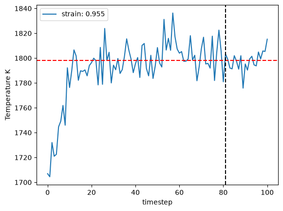
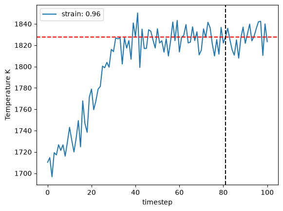
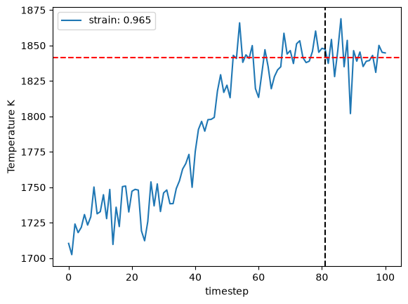
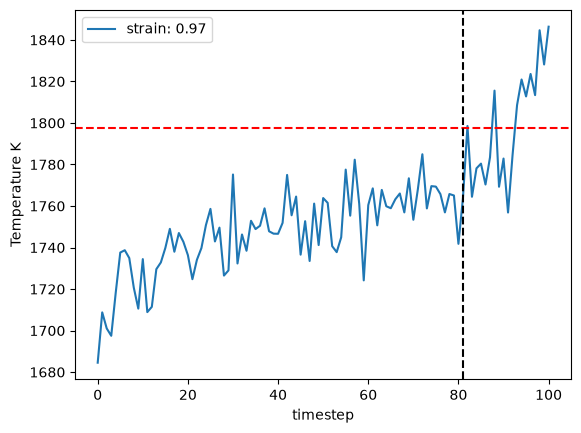
1780.433720977623 1783.4380752956695

temperature_next, temperature_mean, temperature_left, temperature_right

(np.float64(1780.433720977623),
 np.float64(1707.5467248342034),
 np.float64(1691.9751845352537),
 np.float64(1723.1182651331528))

Step 3: validate convergence and refine the numerical settings

validate_convergence() checks whether the temperature predicted in Step 2 (temperature_next) lies inside the window [temperature_left, temperature_right] also computed in Step 2 - i.e. within boundary_value of the actual temperature range spanned by the strain points kept for the fit, meaning the zero-pressure extrapolation was not made from a wildly out-of-range fit. While that holds, the numerical settings are progressively tightened by taking the next entry of timestep_lst, fit_range_lst and nve_run_time_steps_lst (defined in the Configuration section), so later iterations run longer, less strained simulations for a more accurate prediction.

It also records this iteration’s result in step_dict, writes it to output.json, and sets convergence_goal_achieved once the temperature prediction changes by less than convergence_criterion between two consecutive iterations at the tightest settings.

output = validate_convergence(
    temperature_left=temperature_left,
    temperature_next=temperature_next,
    temperature_right=temperature_right,
    enable_iteration=enable_iteration,
    timestep_iter=timestep_iter,
    timestep_lst=project_parameter['timestep_lst'],
    timestep=timestep,
    fit_range_iter=fit_range_iter,
    fit_range_lst=project_parameter['fit_range_lst'],
    fit_range=fit_range,
    nve_run_time_steps_iter=nve_run_time_steps_iter,
    nve_run_time_steps_lst=project_parameter['nve_run_time_steps_lst'],
    nve_run_time_steps=nve_run_time_steps,
    strain_result_lst=strain_result_lst,
    pressure_result_lst=pressure_result_lst,
    step_count=step_count,
    step_dict=step_dict,
    boundary_value=project_parameter['boundary_value'],
    ratio_boundary=project_parameter['ratio_boundary'],
    convergence_goal=project_parameter['convergence_criterion'],
    output_file=output_file
)
convergence_goal_achieved, enable_iteration, step_count, step_dict, timestep, fit_range, nve_run_time_steps, boundary_value, ratio_boundary, temperature_next, center = output

step_dict[step_count]

{'timestep': 2,
 'fit_range': 0.05,
 'nve_run_time_steps': 25000,
 'boundary_value': 0.25,
 'ratio_boundary': 0.25,
 'temperature_next': np.float64(1780.433720977623),
 'center': np.float64(0.94)}

convergence_goal_achieved

False

Step 4: full cycle, predict the final melting point

Step 2 and Step 3 are repeated - each iteration reproducing the same kind of plots described under Step 2 - until convergence_goal_achieved is True (with at least 3 iterations run) or 10 iterations have been reached. output.json is rewritten after every iteration, so this loop is safe to interrupt and resume: rerunning the notebook picks up step_dict from output.json via the reload cell in the Configuration section instead of recomputing already finished iterations. The final cells below print the complete iteration history and plot how the temperature prediction converges over the loop.

temperature_estimate_lst, temperature_calculated_lst = [], []
while len(temperature_calculated_lst) < 3 or not convergence_goal_achieved and len(temperature_calculated_lst) < 10:
    temperature_estimate_lst.append(temperature_next)
    temperature_next, temperature_mean, temperature_left, temperature_right, strain_result_lst, pressure_result_lst = run_interface_iteration(
        basis=basis_minimize_vol.repeat([1,1,2]),
        temperature_next=temperature_next,
        project_parameter=project_parameter,
        project_path=project_path,
        timestep=timestep,
        nve_run_time_steps=nve_run_time_steps,
        fit_range=fit_range,
        center=center,
        debug_plot=True,
        lmp_command=lmp_command,
    )
    print(temperature_next, temperature_mean, temperature_left, temperature_right)
    output = validate_convergence(
        temperature_left=temperature_left,
        temperature_next=temperature_next,
        temperature_right=temperature_right,
        enable_iteration=enable_iteration,
        timestep_iter=timestep_iter,
        timestep_lst=project_parameter['timestep_lst'],
        timestep=timestep,
        fit_range_iter=fit_range_iter,
        fit_range_lst=project_parameter['fit_range_lst'],
        fit_range=fit_range,
        nve_run_time_steps_iter=nve_run_time_steps_iter,
        nve_run_time_steps_lst=project_parameter['nve_run_time_steps_lst'],
        nve_run_time_steps=nve_run_time_steps,
        strain_result_lst=strain_result_lst,
        pressure_result_lst=pressure_result_lst,
        step_count=step_count,
        step_dict=step_dict,
        boundary_value=project_parameter['boundary_value'],
        ratio_boundary=project_parameter['ratio_boundary'],
        convergence_goal=project_parameter['convergence_criterion'],
        output_file=output_file,
    )
    convergence_goal_achieved, enable_iteration, step_count, step_dict, timestep, fit_range, nve_run_time_steps, boundary_value, ratio_boundary, temperature_next, center = output
    print(step_dict[step_count])
    temperature_calculated_lst.append(temperature_next)

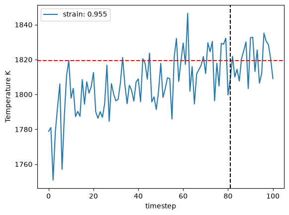
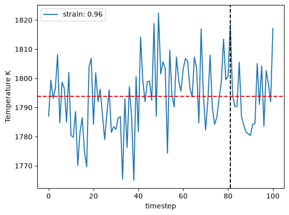
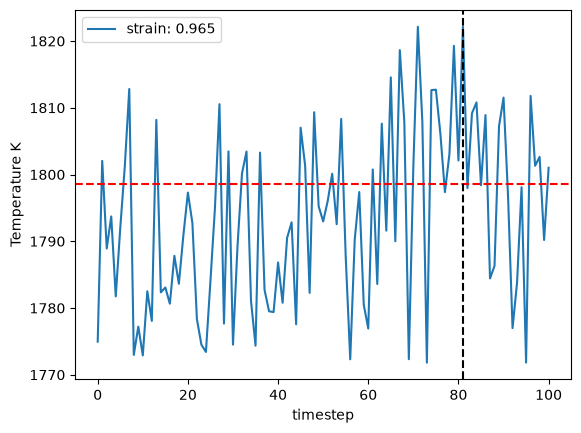
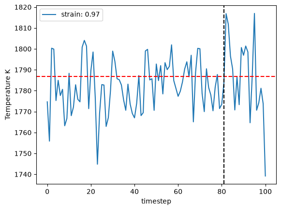
1790.2568639609863 1790.0654397918324
1790.2568639609863 1777.5950240126933 1767.1095667154723 1788.0804813099144
{'timestep': 2, 'fit_range': 0.05, 'nve_run_time_steps': 25000, 'boundary_value': 0.25, 'ratio_boundary': 0.25, 'temperature_next': np.float64(1790.2568639609863), 'center': np.float64(0.96)}

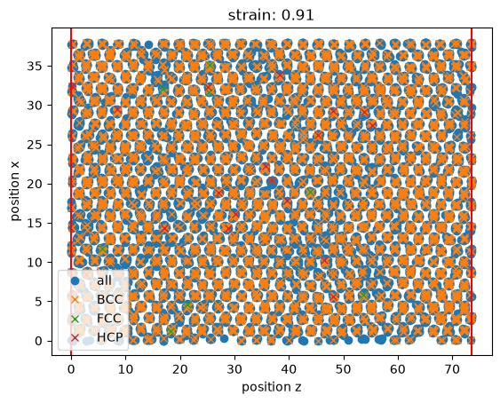
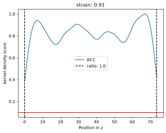
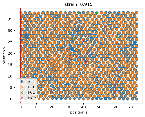
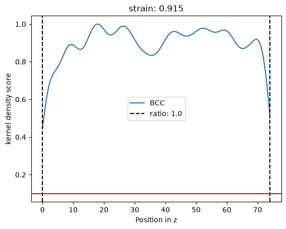
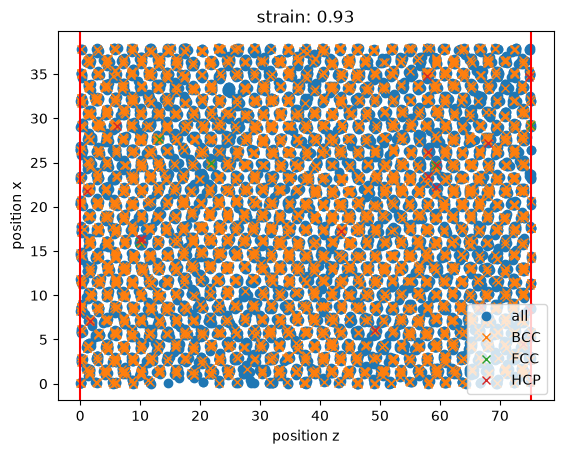
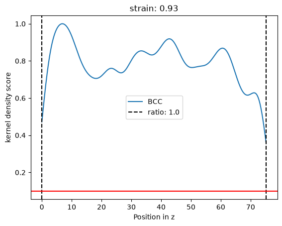
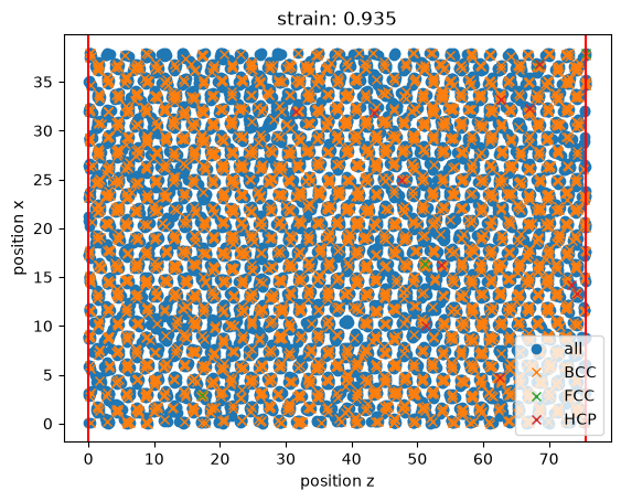
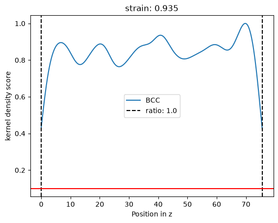
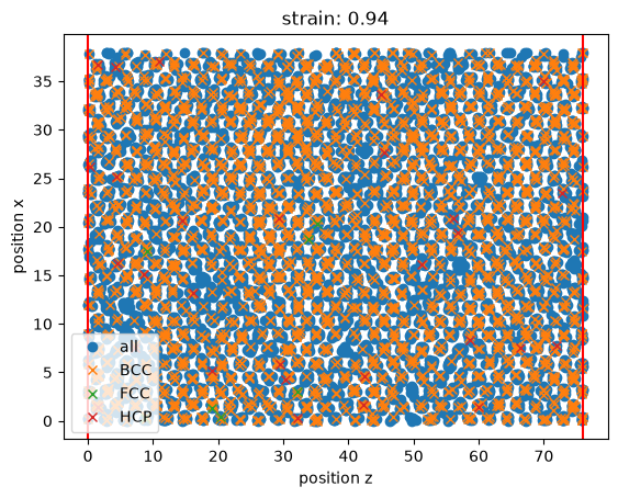
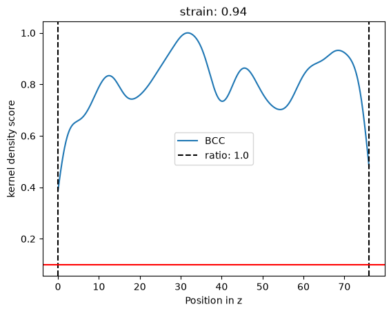
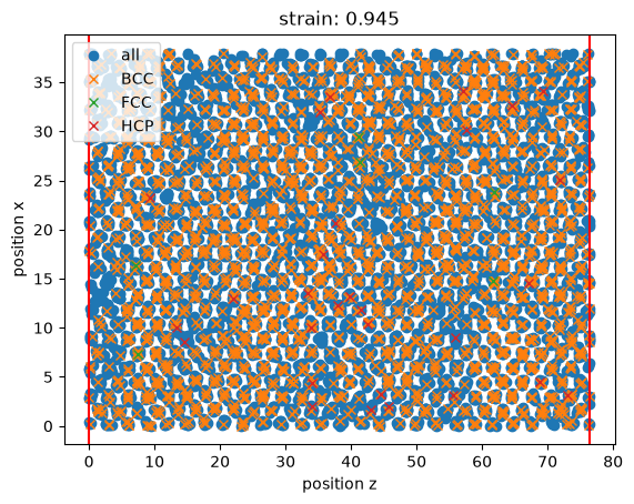
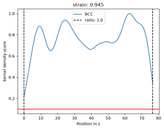
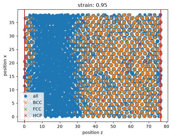
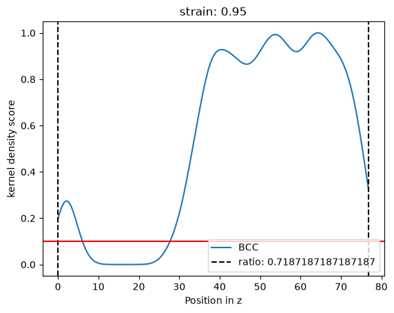
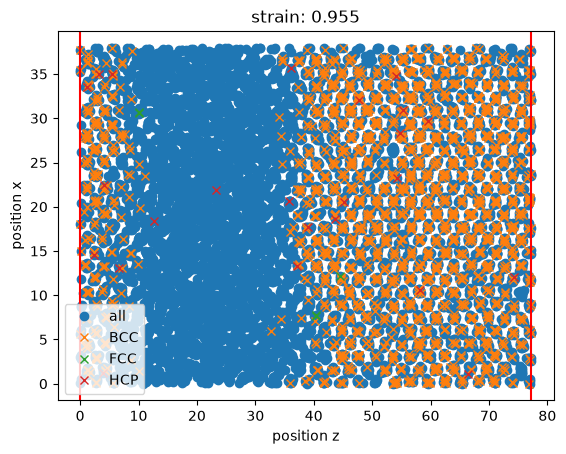
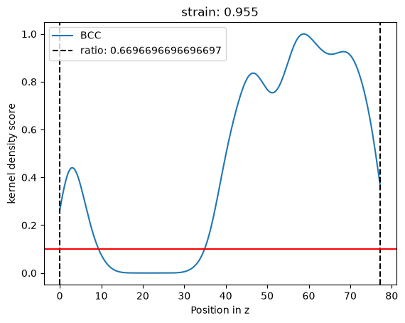
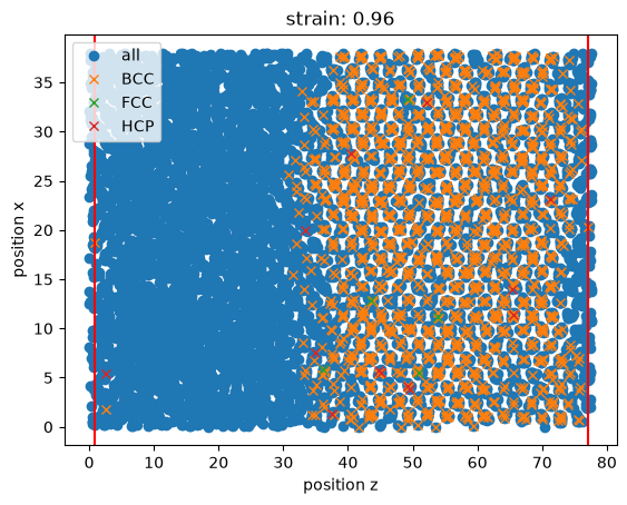
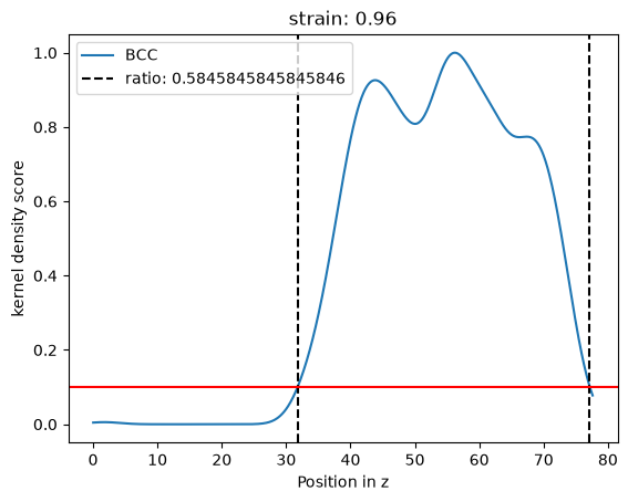
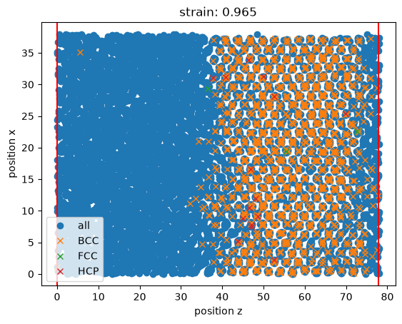
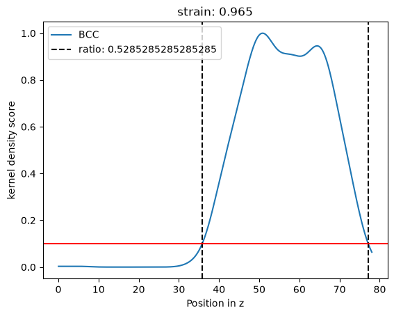
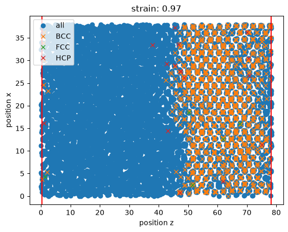
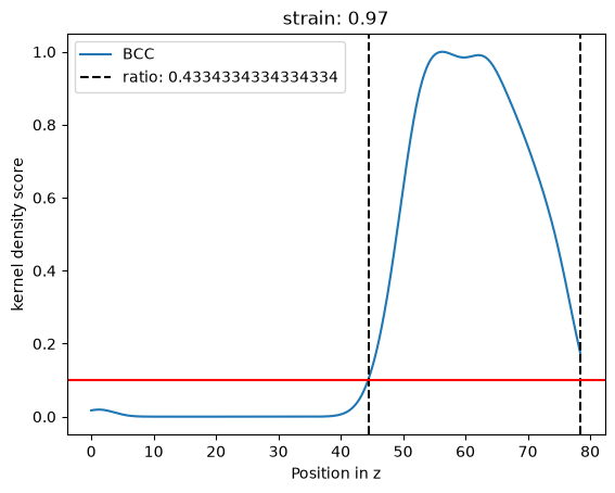
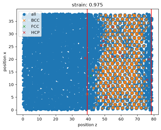
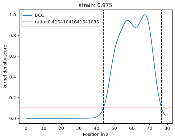
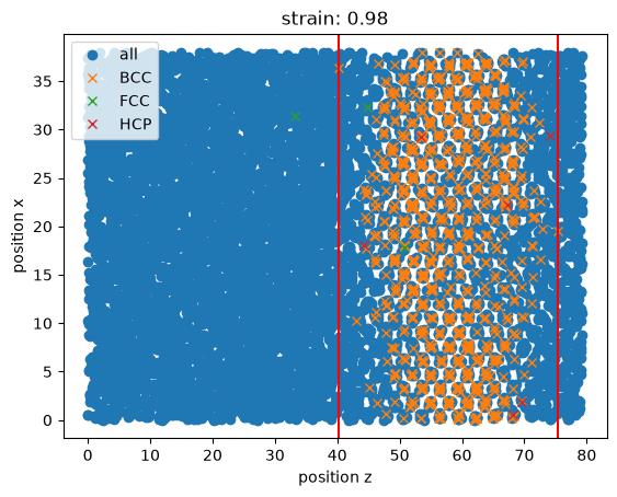
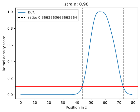
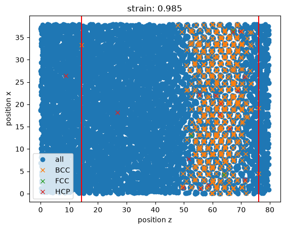
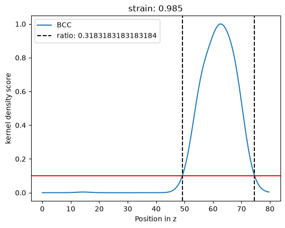
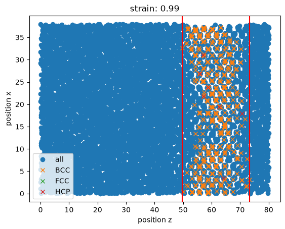
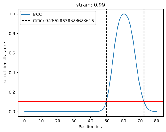
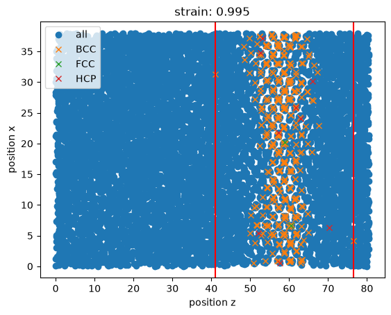
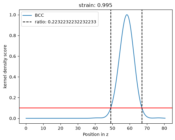
/home/jan/projects/pyiron_meltingpoint/src/interfacemethod/plot.py:158: UserWarning: No artists with labels found to put in legend.  Note that artists whose label start with an underscore are ignored when legend() is called with no argument.
  plt.legend()

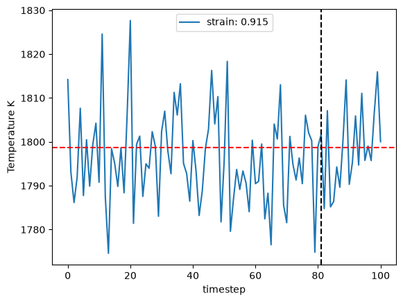
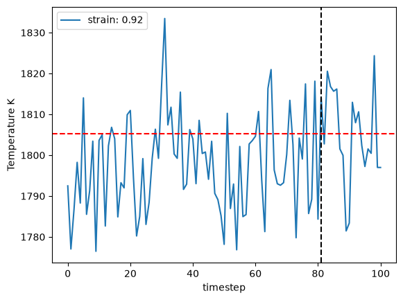
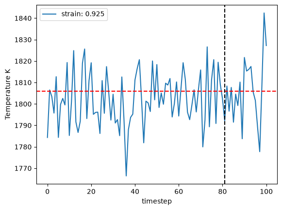
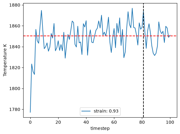
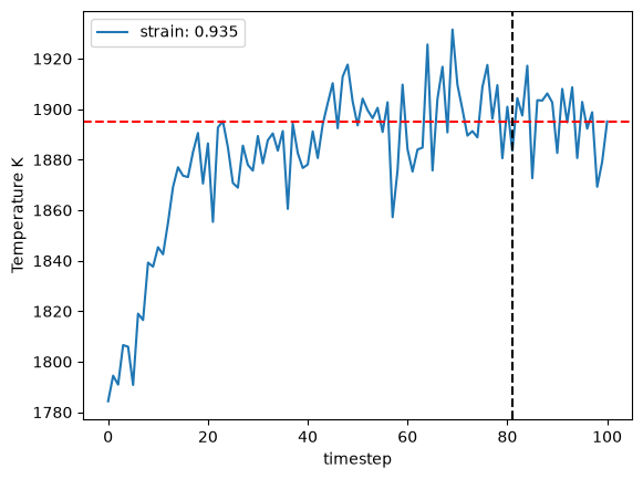
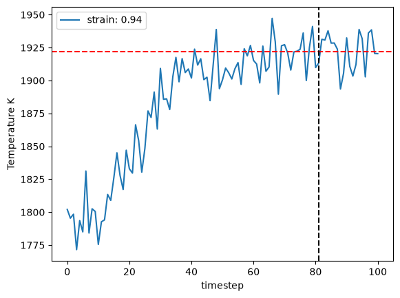
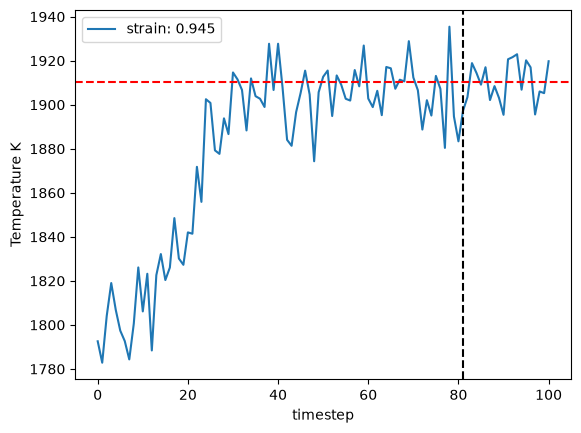
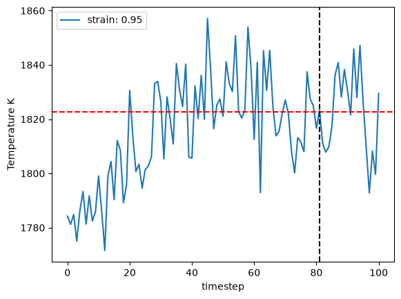
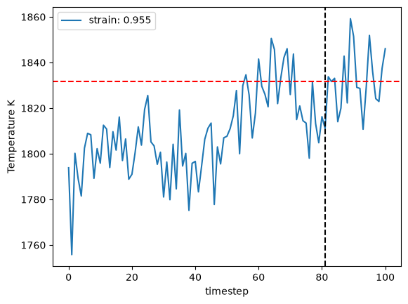
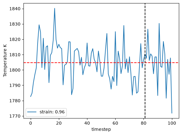
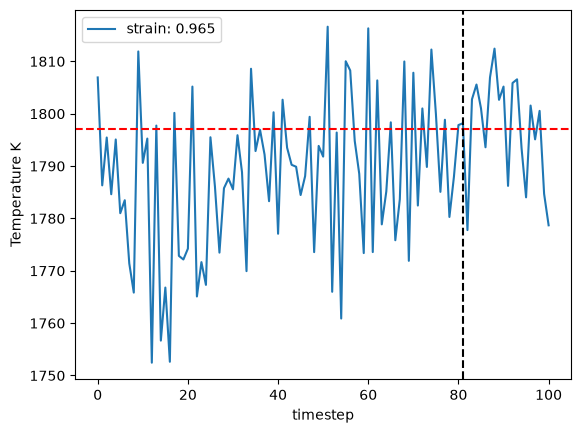
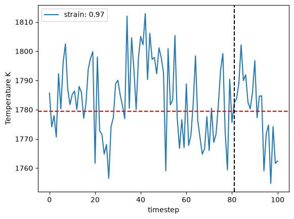
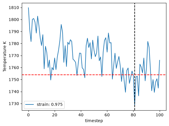
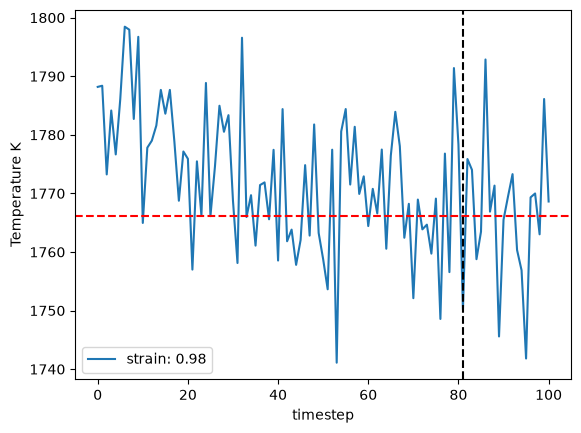
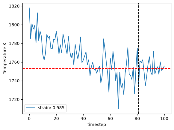
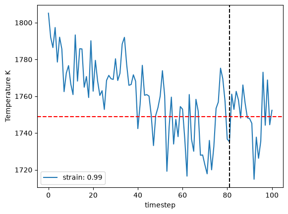
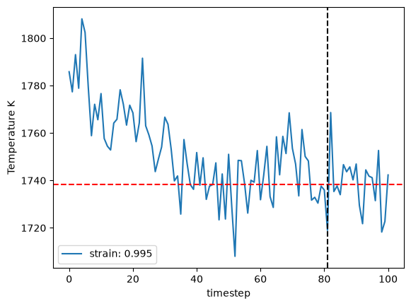
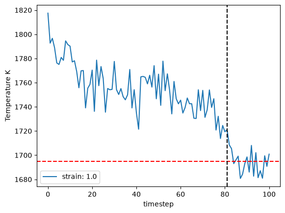
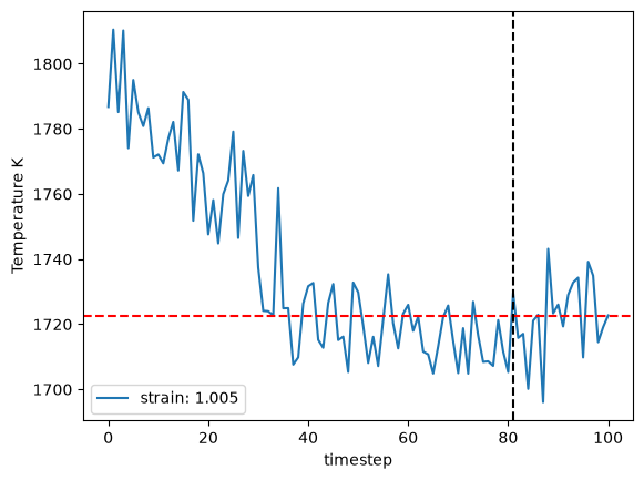
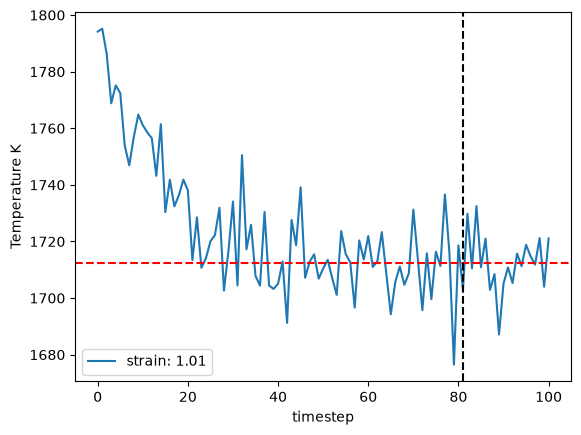
1791.732958036235 1791.7192242312833
1791.732958036235 1790.3757358574221 1769.66514501417 1811.086326700674
{'timestep': 2, 'fit_range': 0.01, 'nve_run_time_steps': 20000, 'boundary_value': 0.25, 'ratio_boundary': 0.25, 'temperature_next': np.float64(1791.732958036235), 'center': np.float64(0.97)}

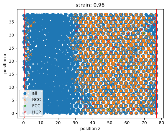
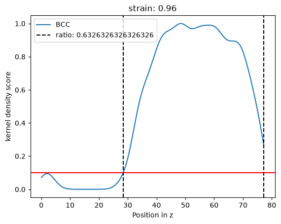
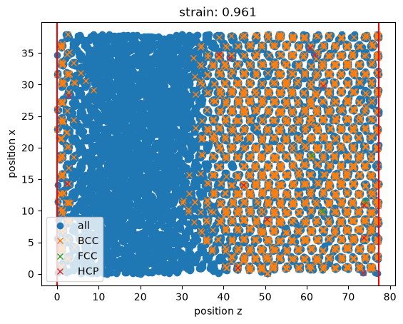
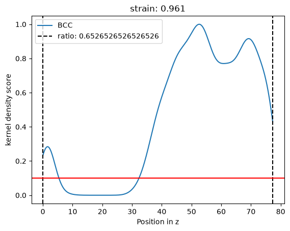
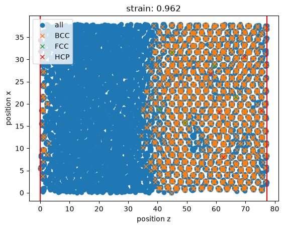
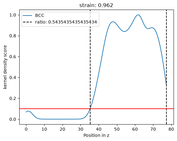
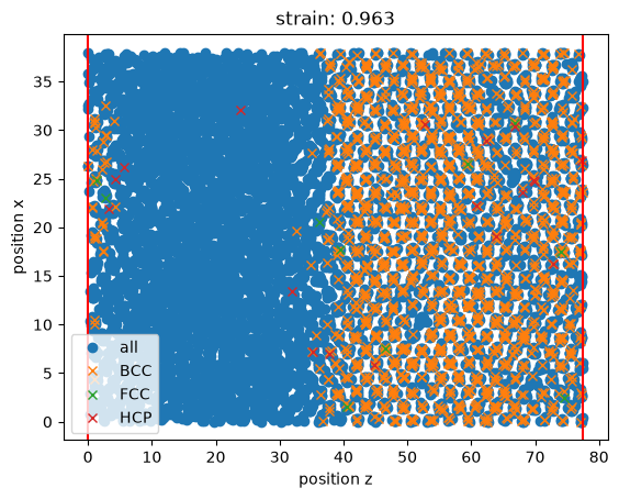
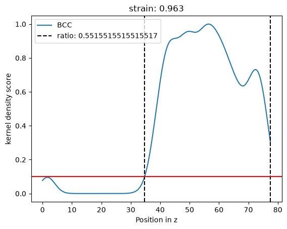
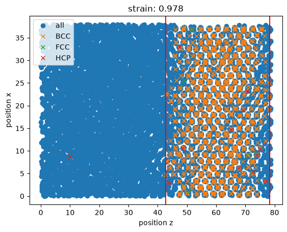
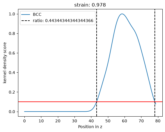
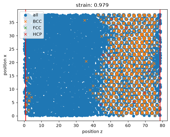
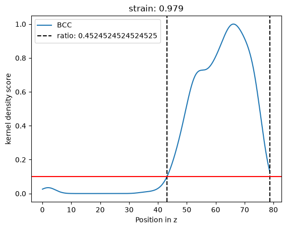
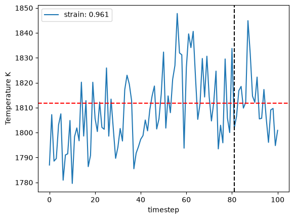
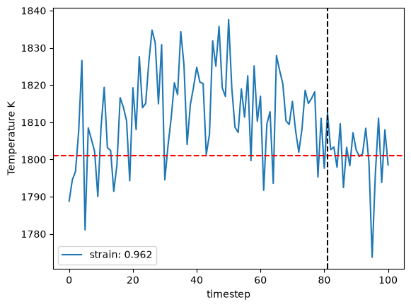
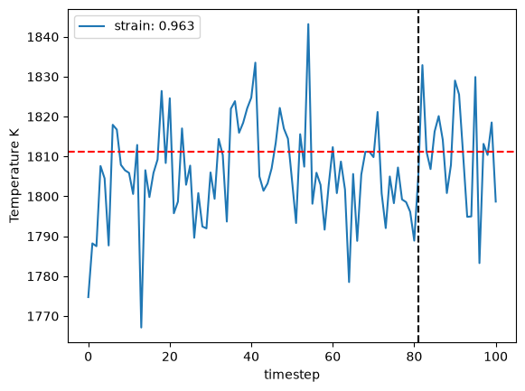
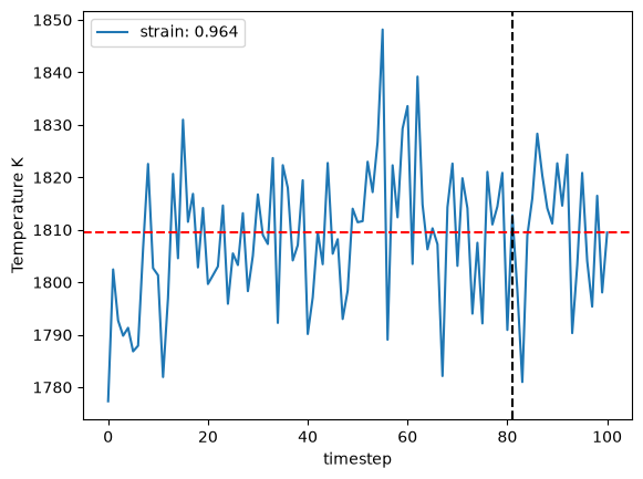
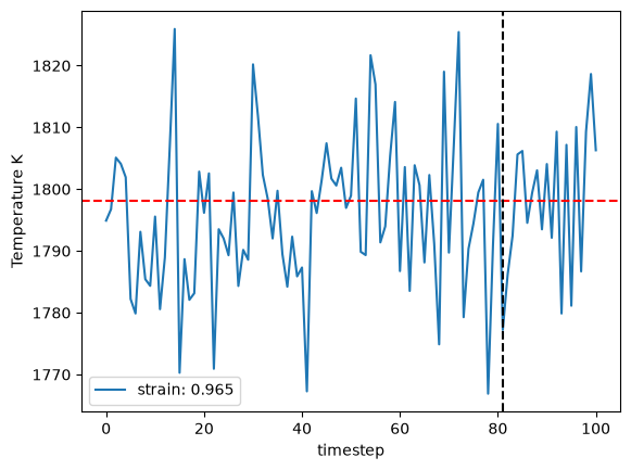
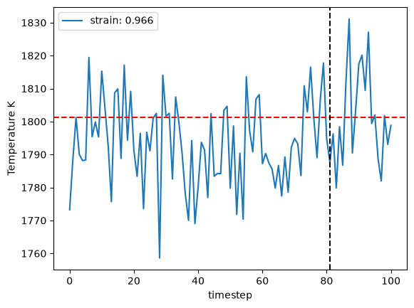
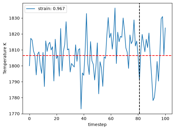
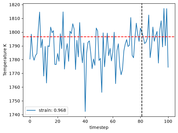
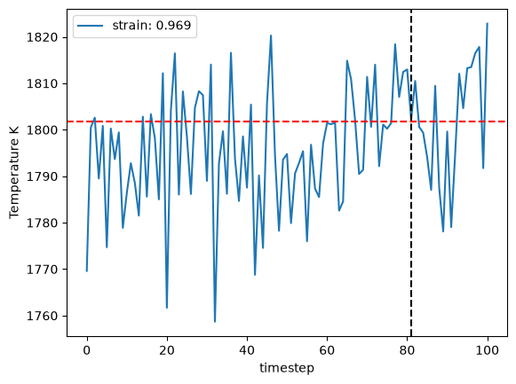
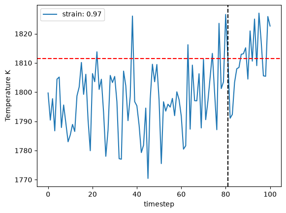
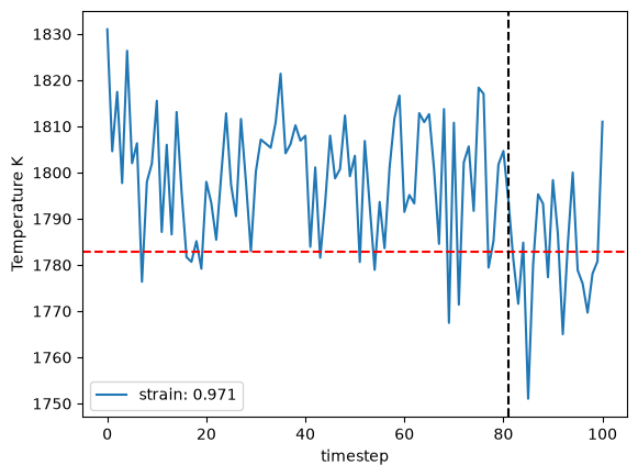
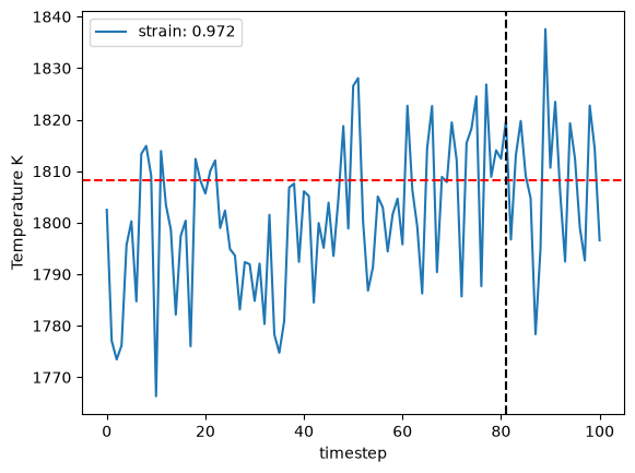
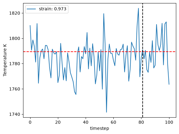
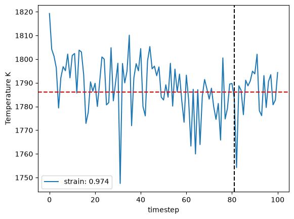
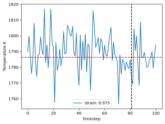
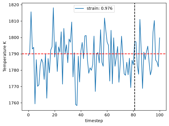
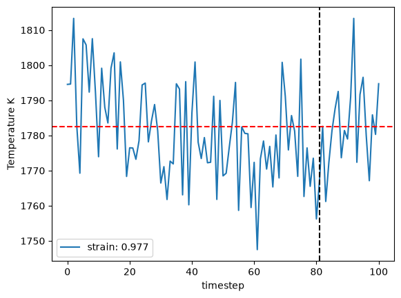
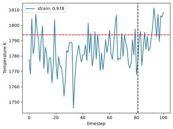
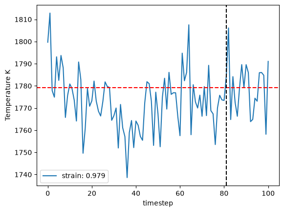
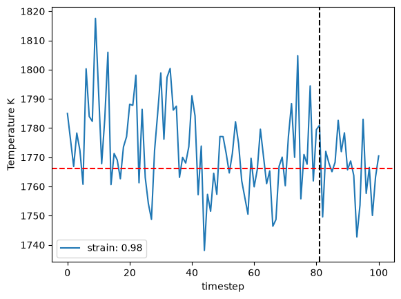
1796.453294409365 1796.4281243385947
1796.453294409365 1795.5598502710138 1780.8361619445845 1810.283538597443
{'timestep': 1, 'fit_range': 0.01, 'nve_run_time_steps': 50000, 'boundary_value': 0.25, 'ratio_boundary': 0.25, 'temperature_next': np.float64(1796.453294409365), 'center': np.float64(0.97)}

1791.4306230865327 1791.2710438874194
1791.4306230865327 1801.8344973853361 1780.7837309724841 1822.8852637981881
{'timestep': 1, 'fit_range': 0.01, 'nve_run_time_steps': 50000, 'boundary_value': 0.25, 'ratio_boundary': 0.25, 'temperature_next': np.float64(1791.4306230865327), 'center': np.float64(0.97)}

1792.2218913908498 1792.4474520200665
1792.2218913908498 1777.91064511217 1760.1134642549946 1795.7078259693453
{'timestep': 1, 'fit_range': 0.01, 'nve_run_time_steps': 50000, 'boundary_value': 0.25, 'ratio_boundary': 0.25, 'temperature_next': np.float64(1792.2218913908498), 'center': np.float64(0.97)}

if not os.path.exists(output_file):
    with open(output_file, 'w') as f:
        json.dump(step_dict, f)

step_dict

{0: {'temperature_next': 1711},
 1: {'timestep': 2,
  'fit_range': 0.05,
  'nve_run_time_steps': 25000,
  'boundary_value': 0.25,
  'ratio_boundary': 0.25,
  'temperature_next': np.float64(1780.433720977623),
  'center': np.float64(0.94)},
 2: {'timestep': 2,
  'fit_range': 0.05,
  'nve_run_time_steps': 25000,
  'boundary_value': 0.25,
  'ratio_boundary': 0.25,
  'temperature_next': np.float64(1790.2568639609863),
  'center': np.float64(0.96)},
 3: {'timestep': 2,
  'fit_range': 0.01,
  'nve_run_time_steps': 20000,
  'boundary_value': 0.25,
  'ratio_boundary': 0.25,
  'temperature_next': np.float64(1791.732958036235),
  'center': np.float64(0.97)},
 4: {'timestep': 1,
  'fit_range': 0.01,
  'nve_run_time_steps': 50000,
  'boundary_value': 0.25,
  'ratio_boundary': 0.25,
  'temperature_next': np.float64(1796.453294409365),
  'center': np.float64(0.97)},
 5: {'timestep': 1,
  'fit_range': 0.01,
  'nve_run_time_steps': 50000,
  'boundary_value': 0.25,
  'ratio_boundary': 0.25,
  'temperature_next': np.float64(1791.4306230865327),
  'center': np.float64(0.97)},
 6: {'timestep': 1,
  'fit_range': 0.01,
  'nve_run_time_steps': 50000,
  'boundary_value': 0.25,
  'ratio_boundary': 0.25,
  'temperature_next': np.float64(1792.2218913908498),
  'center': np.float64(0.97)}}

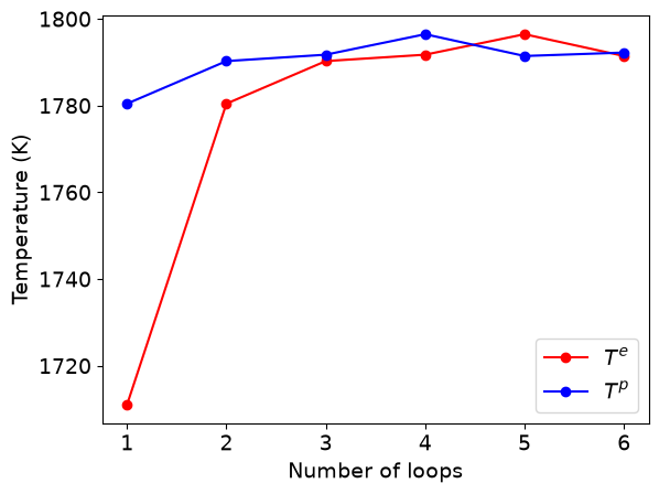
The plot below shows, for every completed iteration of Step 4, the temperature it was given as input (\(T^e\), the estimate coming out of the previous iteration) against the temperature Step 2 predicted from it (\(T^p\)). As the interface method converges the two lines approach each other and flatten out at the predicted melting temperature.

#plot the convergence of loop calculations
first_key = list(step_dict.keys())[-1]
second_key = 'temperature_next'
allt = [step_dict[key][second_key] for key in list(step_dict.keys())]
plt.plot(np.arange(1, len(allt)), allt[0:-1], 'ro-', label=r"$T^e$")
plt.plot(np.arange(1, len(allt)), allt[1:], 'bo-', label=r"$T^p$")
plt.legend(fontsize=14)
plt.tick_params(axis='both', labelsize=14)
plt.xlabel('Number of loops', fontsize=14)
plt.ylabel('Temperature (K)', fontsize=14)
plt.show()

for k, v in sorted(step_dict.items()):
    print(k, v)

0 {'temperature_next': 1711}
1 {'timestep': 2, 'fit_range': 0.05, 'nve_run_time_steps': 25000, 'boundary_value': 0.25, 'ratio_boundary': 0.25, 'temperature_next': np.float64(1780.433720977623), 'center': np.float64(0.94)}
2 {'timestep': 2, 'fit_range': 0.05, 'nve_run_time_steps': 25000, 'boundary_value': 0.25, 'ratio_boundary': 0.25, 'temperature_next': np.float64(1790.2568639609863), 'center': np.float64(0.96)}
3 {'timestep': 2, 'fit_range': 0.01, 'nve_run_time_steps': 20000, 'boundary_value': 0.25, 'ratio_boundary': 0.25, 'temperature_next': np.float64(1791.732958036235), 'center': np.float64(0.97)}
4 {'timestep': 1, 'fit_range': 0.01, 'nve_run_time_steps': 50000, 'boundary_value': 0.25, 'ratio_boundary': 0.25, 'temperature_next': np.float64(1796.453294409365), 'center': np.float64(0.97)}
5 {'timestep': 1, 'fit_range': 0.01, 'nve_run_time_steps': 50000, 'boundary_value': 0.25, 'ratio_boundary': 0.25, 'temperature_next': np.float64(1791.4306230865327), 'center': np.float64(0.97)}
6 {'timestep': 1, 'fit_range': 0.01, 'nve_run_time_steps': 50000, 'boundary_value': 0.25, 'ratio_boundary': 0.25, 'temperature_next': np.float64(1792.2218913908498), 'center': np.float64(0.97)}